
Tiptoe Through the Houston Fire Department Data
A data project
So I have a job that runs every hour and scrapes the HFD incident page so that I can capture all the HFD 911 calls. The job has been running since May 6, 2022. To be honest, I haven’t seen any real obvious patterns, at least geographically. Part of the problem is the resolution. The data is located on the Keymap grid, which are 1x1 mile squares covering the whole area.
This is a first look at that data, just to see what it says.
Read in all the files
Read in the files that have been downloaded so far and do a small amount of cleanup.
filenames <- list.files(path = paste0(path, "Incrementals/"),
pattern="*_table.rds$")
filenames <- paste0(paste0(path, "Incrementals/"),filenames)
df <- filenames %>%
purrr::map_dfr(readRDS) %>%
unique() # get rid of duplicates
df <- df %>%
rename(Incident_type=`Incident Type`,
Cross_street=`Cross Street`,
Call_time=`Call Time(Opened)`,
Combined=`Combined Response`,
Key=`Key Map`)
df <- df %>%
mutate(Incident_type=stringr::str_replace(Incident_type, "fire", "Fire")) %>%
mutate(Incident_type=stringr::str_replace(Incident_type, "FIRE", "Fire")) %>%
mutate(Incident_type=stringr::str_replace(Incident_type, "EVENT", "Event")) %>%
mutate(Incident_type=stringr::str_replace(Incident_type, "Ems", "EMS")) %>%
mutate(Incident_type=stringr::str_replace(Incident_type, "Leaking", "Leak")) %>%
mutate(Incident_type=stringr::str_replace(Incident_type, " on ", " ")) Clean up incident type
Incident type needs a little consolidation, so here I lump a few things together (like Arcing, Wire, and Transformer into Electrical). Yes, there are a lot of dumpster fires.
df_summary <- df %>%
group_by(Incident_type) %>%
summarize(n=n())
df <- df %>%
mutate(Category=case_when(
str_detect(Incident_type, "Dumpster") ~ "Dumpster",
str_detect(Incident_type, "Fire") ~ "Fire",
str_detect(Incident_type, "EMS") ~ "EMS",
str_detect(Incident_type, "Check Patient") ~ "Check Patient",
str_detect(Incident_type, "CRASH") ~ "Crash",
str_detect(Incident_type, "TRAFFIC") ~ "Crash",
str_detect(Incident_type, "Vehicle") ~ "Crash",
str_detect(Incident_type, "Motorcycle") ~ "Crash",
str_detect(Incident_type, "Gas") ~ "Gas Leak",
str_detect(Incident_type, "Alarm") ~ "Alarm",
str_detect(Incident_type, "Smoke Detector") ~ "Alarm",
str_detect(Incident_type, "Pedestrian") ~ "Pedestrian",
str_detect(Incident_type, "Arcing") ~ "Electrical",
str_detect(Incident_type, "Transformer") ~ "Electrical",
str_detect(Incident_type, "Wire") ~ "Electrical",
str_detect(Incident_type, "Electrical") ~ "Electrical",
str_detect(Incident_type, "Elevator") ~ "Elevator",
TRUE ~ "Other"
))
df %>%
group_by(Category) %>%
summarize(n=n()) %>%
arrange(-n) %>%
gt::gt()| Category | n |
|---|---|
| EMS | 132696 |
| Crash | 49077 |
| Fire | 5894 |
| Alarm | 3011 |
| Other | 2138 |
| Check Patient | 1283 |
| Gas Leak | 609 |
| Electrical | 481 |
| Pedestrian | 428 |
| Dumpster | 175 |
| Elevator | 37 |
df_sum <- df %>%
group_by(Key) %>%
summarize(num=n())Attach Keymaps and Census Data
Many of the incidents are located only by Keymap code. Some instead have an address. For those, we will try to geocode the address and then attach a Keymap code for that address.
When that is done, we will then attach some census data to the incidents.
library(postmastr)
library(GeocodeHou)
googlecrs <- "EPSG:4326" # lat long
CoH_crs <- "EPSG:2278" # X-Y
Keyfiles <- readRDS(paste0("/home/ajackson/Dropbox/Rprojects/Curated_Data_Files/Keymaps/", "Trans_Tab.rds"))
Keypolys <- readRDS(paste0("/home/ajackson/Dropbox/Rprojects/Curated_Data_Files/Keymaps/", "Trans_Tab_Poly_ll.rds"))
df <- df %>%
mutate(Seq=row_number()) %>%
mutate(Time=lubridate::hour(lubridate::mdy_hm(Call_time))) %>%
mutate(Daytime=if_else(Time<6|Time>18,FALSE, TRUE))
# Make begin and end date strings
Date_stamp <- lubridate::stamp_date("Jan 17, 1999")
Beg_date <- Date_stamp(min(lubridate::mdy_hm(df$Call_time)))
End_date <- Date_stamp(max(lubridate::mdy_hm(df$Call_time)))
Time_period <- paste("From", Beg_date, "to", End_date)
dfnew <- left_join(df, Keyfiles, by="Key")
dfnew <- sf::st_as_sf(dfnew)
# Many have no Key, but some have an address. Geocode and then match to Key
foo <- dfnew %>%
filter(Key=="") %>%
filter(!Address=="") %>%
mutate(Zip="77000") %>% # bogus zipcode
mutate(St_num=stringr::str_extract(Address, "^\\d*")) %>%
filter(!St_num=="")
foo <- pm_identify(foo, var="Address") # add ID fields
foo2 <- pm_prep(foo, var="Address", type="street") # Prep data
foo2 <- pm_houseFrac_parse(foo2)
foo2 <- pm_house_parse(foo2)
foo2 <- pm_streetDir_parse(foo2)
foo2 <- pm_streetSuf_parse(foo2)
foo2 <- pm_street_parse(foo2)
foo2 <- foo2 %>%
mutate(pm.street=str_to_upper(pm.street)) %>%
mutate(pm.streetSuf=str_to_upper(pm.streetSuf)) %>%
mutate(pm.preDir=replace_na(pm.preDir, "")) %>%
mutate(pm.streetSuf=replace_na(pm.streetSuf, ""))
foo <- pm_replace(foo2, source=foo)
match <- NULL
for (i in 1:nrow(foo)){ # match to get zipcode
if (is.na(foo[i,]$pm.street)) {next}
#print(paste("i=",i))
tmp <- GeocodeHou::repair_zipcode(foo[i,]$pm.house,
foo[i,]$pm.preDir,
foo[i,]$pm.street,
foo[i,]$pm.streetSuf,
foo[i,]$Zip)
if (tmp$Success){ # success
#print(paste("Success", tmp$Lat, tmp$Lon, tmp$New_zipcode))
match <- cbind(foo[i,], tmp) %>%
select(pm.house, pm.preDir, pm.street, pm.streetSuf, New_zipcode, Seq, Lat, Lon) %>%
rbind(., match)
} else { # Fail exact match
#print(paste("Failed", tmp$Fail))
}
}
# Use lat long to find which keymap key
match_ll <- st_as_sf(match, coords=c("Lon", "Lat"), crs=googlecrs)
aaa <- st_intersects(st_transform(match_ll, crs=CoH_crs),
st_transform(Keypolys, crs=CoH_crs),
sparse=TRUE)
aaab <-Keypolys[unlist(aaa),] %>%
st_drop_geometry() %>%
select(Key) %>%
bind_cols(., st_drop_geometry(match_ll)) %>%
select(Key, Seq)
mask <- dfnew$Seq %in% aaab$Seq
dfnew[dfnew$Seq %in% aaab$Seq,]$Key <- aaab$Key
# Drop rows without a Keymap code
dfnew <- dfnew %>%
filter(!Key=="")
# Sum up by Keymap, daytime or night, and Category
dfnew_sum <- dfnew %>%
group_by(Category, Key, Daytime) %>%
summarise(n=n())
# Attach some census data
censuspath <- "/home/ajackson/Dropbox/Rprojects/Curated_Data_Files/Census_data/"
censusKey <- readRDS(paste0(censuspath, "Census_data_by_Keymap_2020.rds")) %>%
select(Key, Pop, Pop_white, Pop_black, Pop_asian, Pop_hispanic, Pop_not_hisp,
Pop_blk_grpE, Aggreg_incE) %>%
mutate(Avg_income=na_if(Aggreg_incE/Pop_blk_grpE, Inf))
df_all <- left_join(dfnew_sum, censusKey, by="Key")
df_all_poly <- left_join(st_drop_geometry(df_all), Keypolys, by="Key")
df_all_poly <- sf::st_as_sf(df_all_poly) %>% filter(!is.null(Poly[[1]]))Crossplots
Looking at EMS calls, since I want to compare those to the income to look for anomalies, we restrict the time to night-time since that is when income is meaningful - people are largely at home in bed.
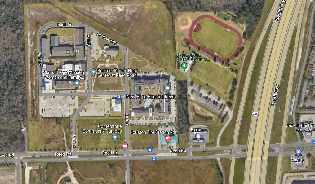
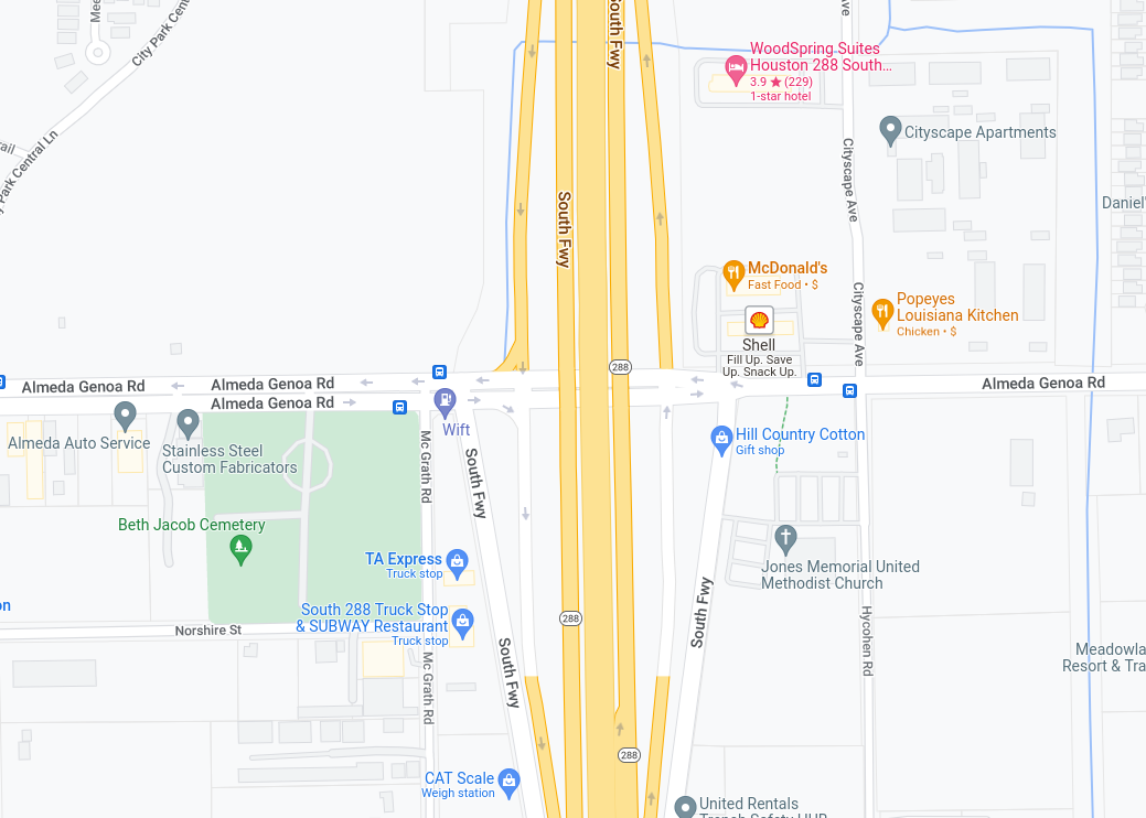
So what about the outliers? The Keymap squares are a bit unwieldy, so I can only guess at what is influencing each square (they are one mile square), but here are my guesses for the top three outliers.
Star of Hope Shelter and New Hope Housing are really the only occupied buildings in the area.
The Cityscape apartment complex has been a problem for the city for some time, there are articles in the Chronicle describing the problems.
Really have no idea. Mostly an industrial area. There are the Fountains at Almeda apartments, but no news stories about them. A mystery.
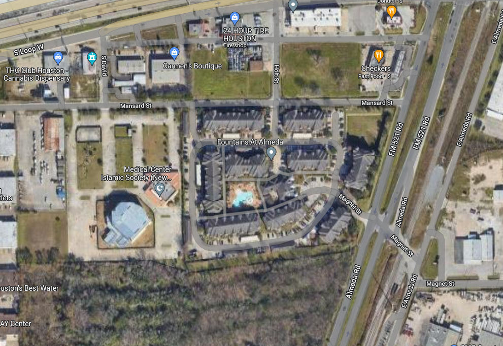
This reveals a general problem with much of this analysis. The one mile square resolution of the data is just too coarse to make many good conclusions.
df_EMS_day <- df_all_poly %>%
filter(Category=="EMS") %>%
filter(n>10) %>%
filter(Daytime)
df_EMS_nite <- df_all_poly %>%
filter(Category=="EMS") %>%
filter(n>10) %>%
filter(!Daytime)
foo <- df_EMS_nite %>%
filter(!is.na(Pop)) %>%
filter(Pop>100) %>%
mutate(percap=n/Pop)
foo %>%
ggplot(aes(y=Avg_income, x=percap)) +
geom_point() +
labs(title="EMS Incidents Per Capita vs. Average Income",
subtitle=Time_period,
x="Incidents per capita",
y = "Average Income in Dollars")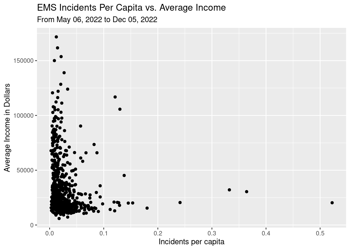
Some maps of polygons
Let’s look at EMS calls in daytime, nighttime, both totals and per capita.
I don’t see any obvious patterns.
# Produces a ggplot object
bbox <- tmaptools::bb(osmdata::getbb(place_name = "Houston"))
Base_basemapR <- basemapR::base_map(bbox, basemap="mapnik", increase_zoom=2)## attribution: © <a href="https://www.openstreetmap.org/copyright">OpenStreetMap</a> contributors# First just raw numbers
df_EMS <- df_all_poly %>%
filter(Category=="EMS") %>%
filter(n>10)
df_EMS_day <- df_EMS %>%
filter(Daytime)
df_EMS_day %>%
filter(n>50) %>%
ggplot() +
Base_basemapR +
geom_sf(aes(fill=n), alpha=0.3)+
scale_fill_gradientn(colors=rainbow(5), limits=c(50,300)) +
ggtitle("Total Daytime EMS Calls per Keymap Square",
subtitle=Time_period)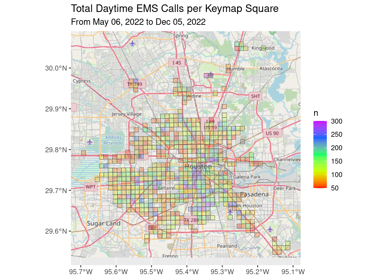
df_EMS_nite <- df_EMS %>%
filter(!Daytime)
df_EMS_nite %>%
filter(n>50) %>%
ggplot() +
Base_basemapR +
geom_sf(aes(fill=n), alpha=0.3)+
scale_fill_gradientn(colors=rainbow(5), limits=c(50,300))+
ggtitle("Total Nighttime EMS Calls per Keymap Square",
subtitle=Time_period)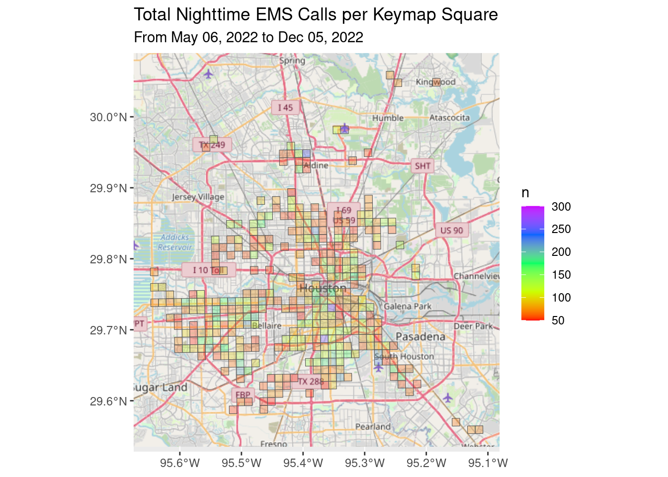
df_EMS %>%
ggplot() +
Base_basemapR +
geom_sf(aes(fill=n), alpha=0.3)+
#scale_fill_gradientn(colors=pal(df_EMS$n))+
scale_fill_gradientn(colors=rainbow(8), limits=c(0,800))+
ggtitle("Total EMS Calls per Keymap Square",
subtitle=Time_period)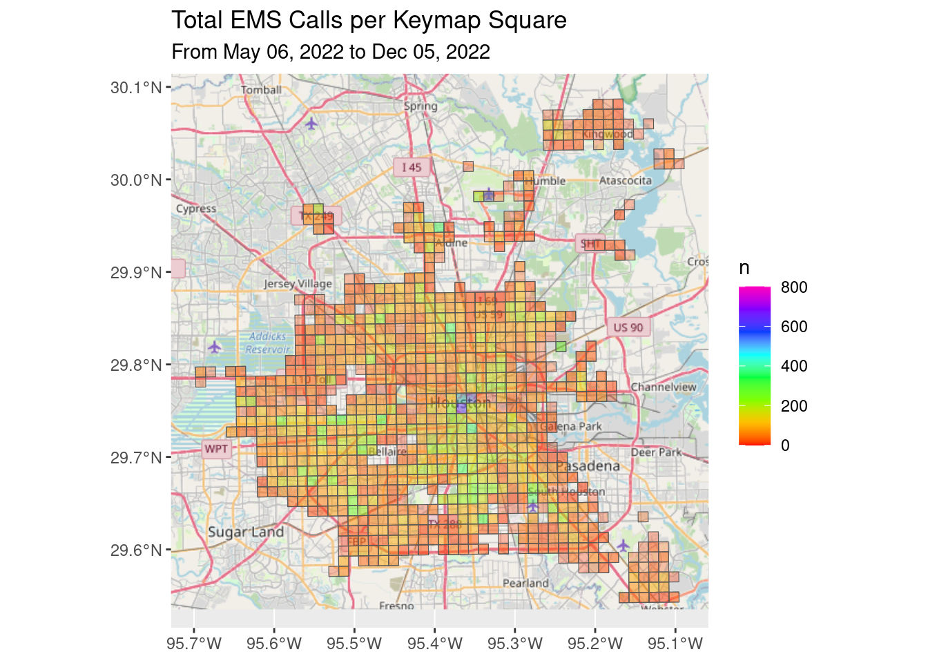
# Let's do per capita
# First the blocks with no people resident
df_EMS %>%
filter(is.na(Pop)) %>%
ggplot() +
Base_basemapR +
geom_sf(aes(fill=n), alpha=0.3)+
scale_fill_gradientn(colors=rainbow(5), limits=c(10,200))+
ggtitle("Blocks with no people (airports, outside county)",
subtitle=Time_period)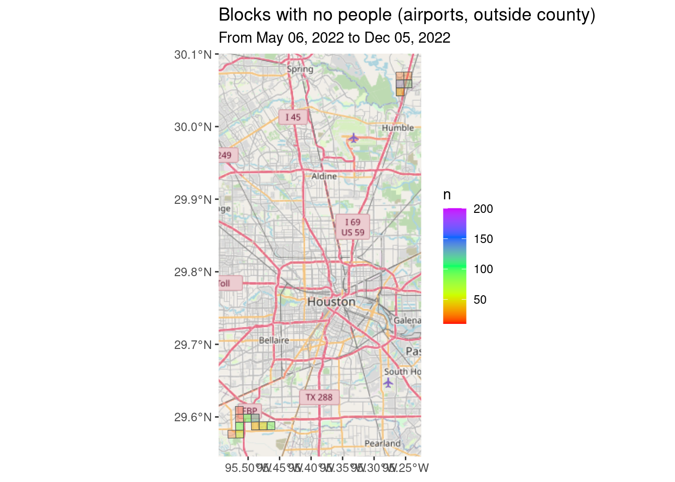
# These are either the airport or outside of Harris County
# Now do per capita
df_EMS_nite %>%
filter(!is.na(Pop)) %>%
mutate(percap=n/Pop) %>%
ggplot() +
Base_basemapR +
geom_sf(aes(fill=percap), alpha=0.3)+
scale_fill_gradientn(colors=rainbow(5), limits=c(0, 0.1))+
ggtitle("Per Capita Nighttime EMS Calls per Keymap Square",
subtitle=Time_period)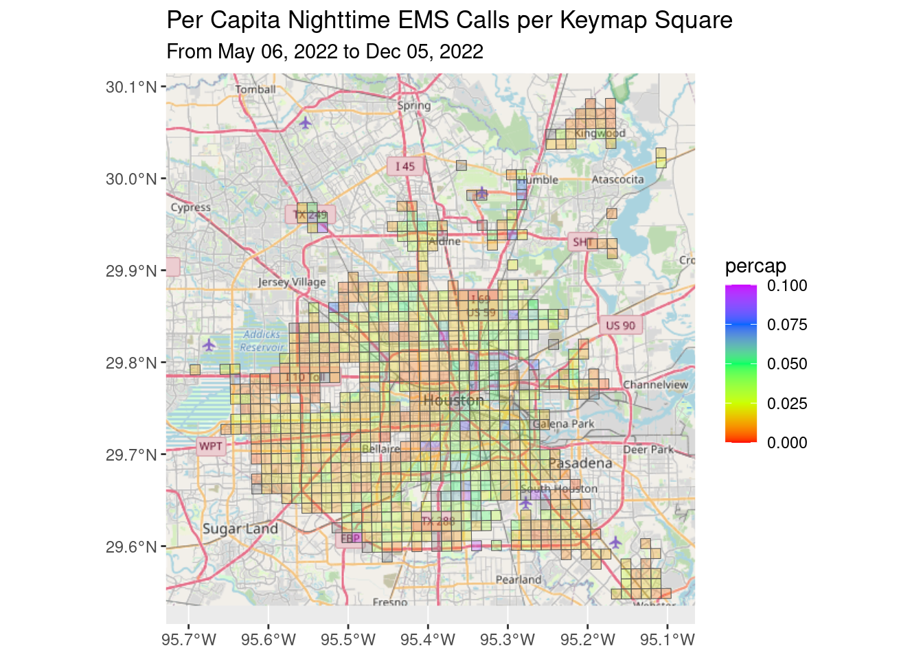
# Let's look at blocks with real population.
df_EMS_nite %>%
filter(!is.na(Pop)) %>%
filter(Pop>1000) %>%
mutate(percap=n/Pop) %>%
filter(percap>0.01) %>%
ggplot() +
Base_basemapR +
geom_sf(aes(fill=percap), alpha=0.3)+
scale_fill_gradientn(colors=rainbow(5), limits=c(0.01, 0.1))+
ggtitle("Per Capita Nighttime EMS Calls per Keymap Square",
subtitle=Time_period)+
labs(subtitle="For Population > 1000 in square") 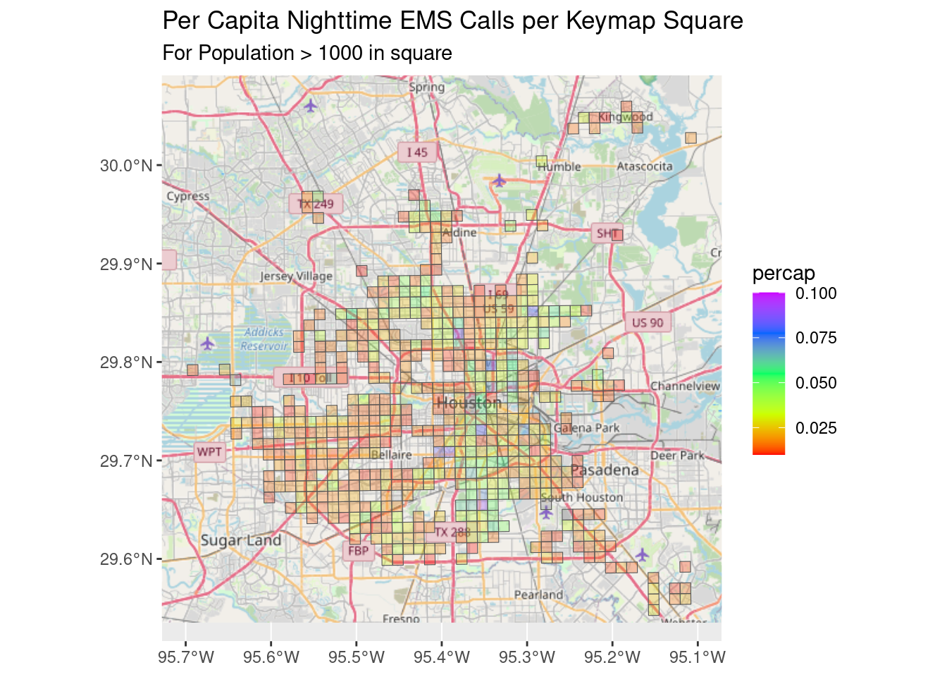
Interactive maps of other incidents
These sort of Leaflet maps are not the best for seeing patterns, but on the other hand, for the most part, I don’t see any particular patterns emerging, except perhaps for crashes. But for that the TxDOT data is probably a better source.
# Stuff to add title to Leaflet map
tag.map.title <- tags$style(HTML("
.leaflet-control.map-title {
transform: translate(-50%,20%);
position: fixed !important;
left: 50%;
text-align: center;
padding-left: 10px;
padding-right: 10px;
background: rgba(255,255,255,0.75);
font-weight: bold;
font-size: 20;
}
"))
title <- tags$div(
tag.map.title, HTML("All Calls"))
dfnew %>%
leaflet() %>%
addTiles() %>%
addMarkers(clusterOptions = markerClusterOptions(),
label=~as.character(Key)) %>%
addControl(title, position = "topright", className="map-title")## Warning in validateCoords(lng, lat, funcName): Data contains 324 rows with
## either missing or invalid lat/lon values and will be ignoredtitle <- tags$div(
tag.map.title, HTML("Dumpster Fires"))
dfnew %>%
filter(str_detect(Incident_type, "Dumpster")) %>%
leaflet() %>%
addTiles() %>%
addMarkers(clusterOptions = markerClusterOptions()) %>%
addControl(title, position = "topright", className="map-title")title <- tags$div(
tag.map.title, HTML("Crashes"))
dfnew %>%
filter(str_detect(Incident_type, "CRASH")) %>%
leaflet() %>%
addTiles() %>%
addMarkers(clusterOptions = markerClusterOptions(),
label=~as.character(Key)) %>%
addControl(title, position = "topright", className="map-title")## Warning in validateCoords(lng, lat, funcName): Data contains 252 rows with
## either missing or invalid lat/lon values and will be ignoredtitle <- tags$div(
tag.map.title, HTML("Fires"))
dfnew %>%
filter(str_detect(Incident_type, "Fire")) %>%
leaflet() %>%
addTiles() %>%
addMarkers(clusterOptions = markerClusterOptions(),
label=~as.character(Key)) %>%
addControl(title, position = "topright", className="map-title")Some final maps
Let’s make nice static maps for the previous categories, just to see what we can see.
df_all_poly %>%
filter(Daytime) %>%
group_by(Key) %>%
summarize(n=sum(n, na.rm = TRUE)) %>%
ggplot() +
Base_basemapR +
geom_sf(aes(fill=n), alpha=0.3)+
scale_fill_gradientn(colors=rainbow(5), limits=c(0.0, 300))+
ggtitle("Total Daytime Calls per Keymap Square",
subtitle=Time_period)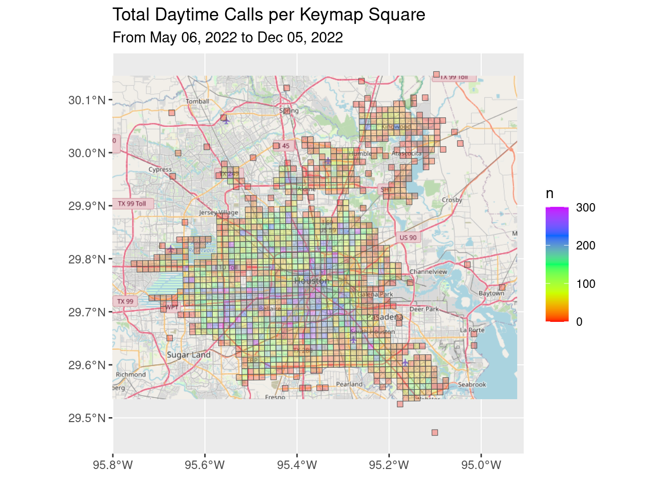
df_all_poly %>%
filter(!Daytime) %>%
group_by(Key) %>%
summarize(n=sum(n, na.rm = TRUE)) %>%
ggplot() +
Base_basemapR +
geom_sf(aes(fill=n), alpha=0.3)+
scale_fill_gradientn(colors=rainbow(5), limits=c(0.0, 200))+
ggtitle("Total Nighttime Calls per Keymap Square",
subtitle=Time_period)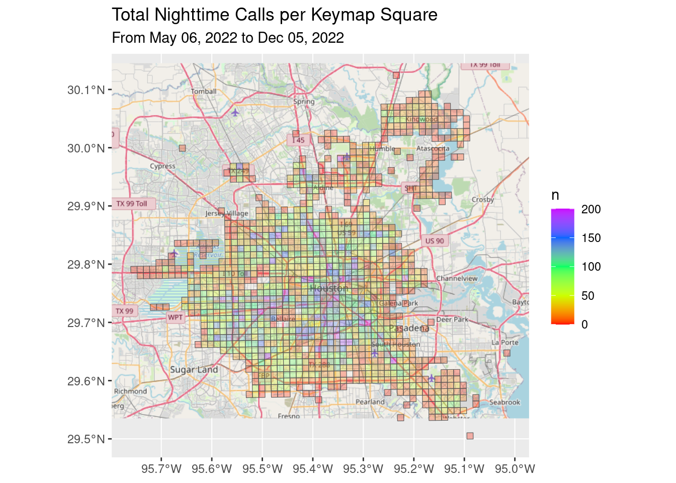
# Dumpster Fires
df_all_poly %>%
filter(str_detect(Category, "Dumpster")) %>%
group_by(Key) %>%
summarize(n=sum(n, na.rm = TRUE)) %>%
ggplot() +
Base_basemapR +
geom_sf(aes(fill=n), alpha=0.3)+
scale_fill_gradientn(colors=rainbow(5), limits=c(1, 4))+
ggtitle("Total Dumpster Fires per Keymap Square",
subtitle=Time_period)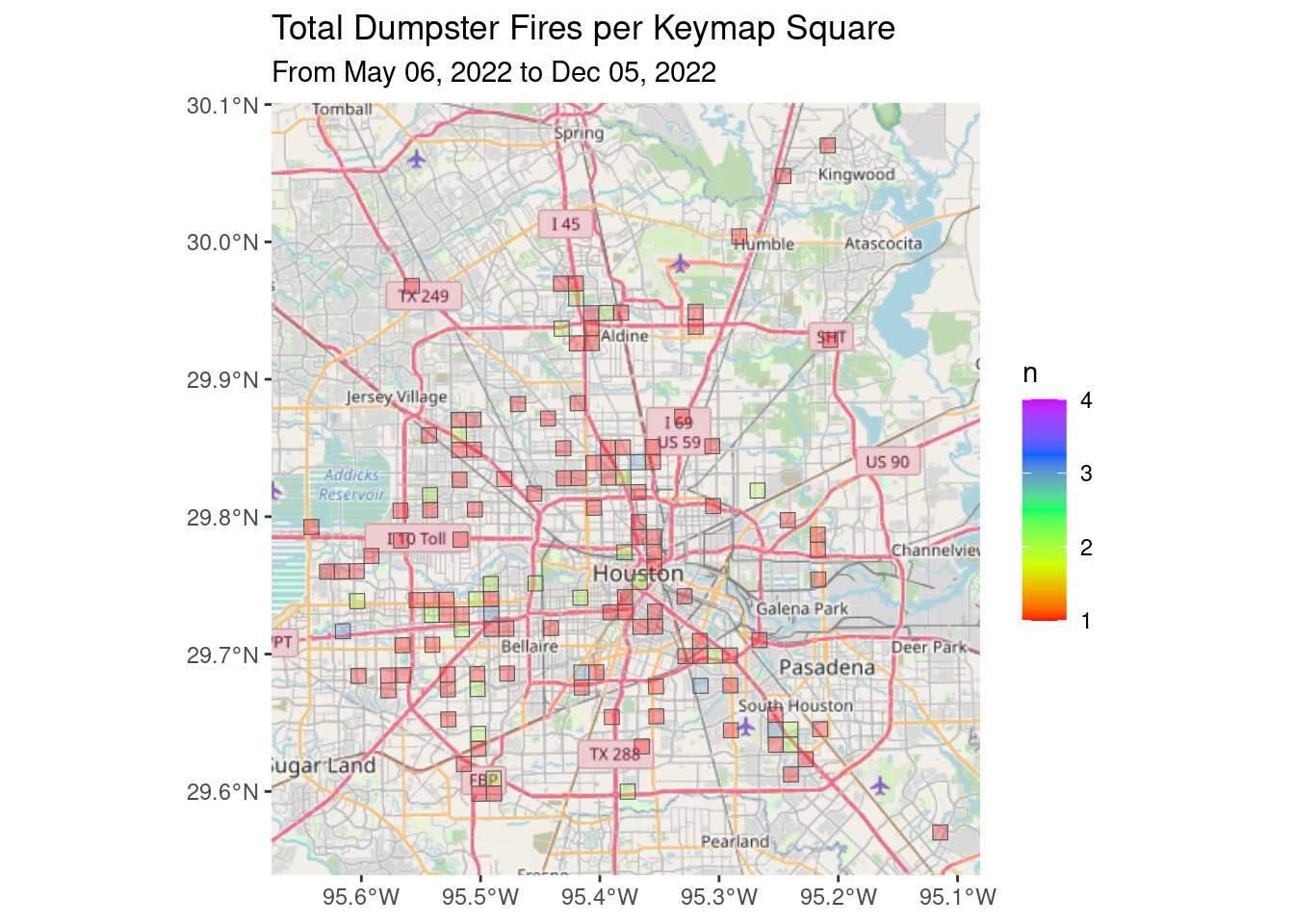
# Crashes
df_all_poly %>%
filter(str_detect(Category, "Crash")) %>%
group_by(Key) %>%
summarize(n=sum(n, na.rm = TRUE)) %>%
ggplot() +
Base_basemapR +
geom_sf(aes(fill=n), alpha=0.3)+
scale_fill_gradientn(colors=rainbow(5), limits=c(1, 200))+
ggtitle("Total Crashes per Keymap Square",
subtitle=Time_period)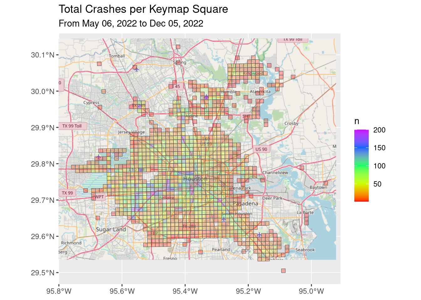
# Fires
df_all_poly %>%
filter(str_detect(Category, "Fire")) %>%
group_by(Key) %>%
summarize(n=sum(n, na.rm = TRUE)) %>%
ggplot() +
Base_basemapR +
geom_sf(aes(fill=n), alpha=0.3)+
scale_fill_gradientn(colors=rainbow(5), limits=c(1, 25))+
ggtitle("Total Fires per Keymap Square",
subtitle=Time_period)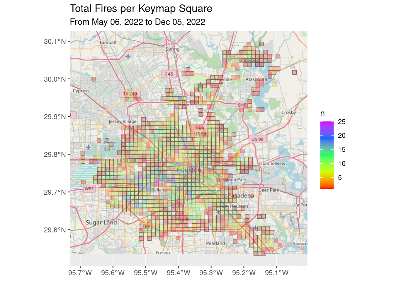
Summary
I haven’t found this data to be very enlightening yet. I’ll have to think about what might be interesting. But this is it for now.