Early Voting Harris County
Let’s take a look at the early voting data for Harris County
Since I already have a bunch of data for Harris county precincts and zipcodes, why not make some use of it?
Setup
path <- "/home/ajackson/Dropbox/Rprojects/Voting/"
BBM <- read_csv(paste0(path, "Cumulative_BBM_1120.csv"),
                col_types = "ccccccccccccccccccccccccccccccccccccccccc")
BBM <- BBM %>%
  mutate(ActivityDate=mdy_hms(ActivityDate)) %>%
  mutate(ActivityDate=force_tz(ActivityDate, tzone = "US/Central")) %>%
  select(ElectionCode:ActivityDate) %>%
  mutate(Ballot_Type="Mail")

EV  <- list.files(path=path, pattern="Cumulative_EV_1120_1*", full.names=TRUE) %>%
  map_df(~read_csv(., col_types = "ccccccccccccccccccccccccccccccccccccccccc"))


EV <- EV %>%
  mutate(ActivityDate=mdy_hms(ActivityDate)) %>%
  mutate(ActivityDate=force_tz(ActivityDate, tzone = "US/Central")) %>%
  select(ElectionCode:ActivityDate) %>%
  mutate(Ballot_Type="Early")

Votes <- rbind(BBM, EV)

VotesByZipDate <- Votes %>%
  mutate(Date=floor_date(ActivityDate, unit="day")) %>%
  group_by(Date, Ballot_Type, VoterZIP) %>%
    summarise(Votes=n()) %>%
  ungroup() %>%
  rename(Zip=VoterZIP) %>%
  drop_na()

###########   registered voters
path <- paste0(path, "HarrisRegisteredVoters/")

files <- dir(path=path, pattern = "*.csv", full.names=TRUE)

Registered <- files %>%
  map_dfr(read_csv, col_types=cols(.default = "c"))

Registered %>%
  filter(Status=="Active") %>%
  mutate(`Effective Date`=mdy(`Effective Date`)) %>%
  filter(!is.na(`Effective Date`)) %>%
  ggplot(aes(`Effective Date`)) +
  geom_histogram()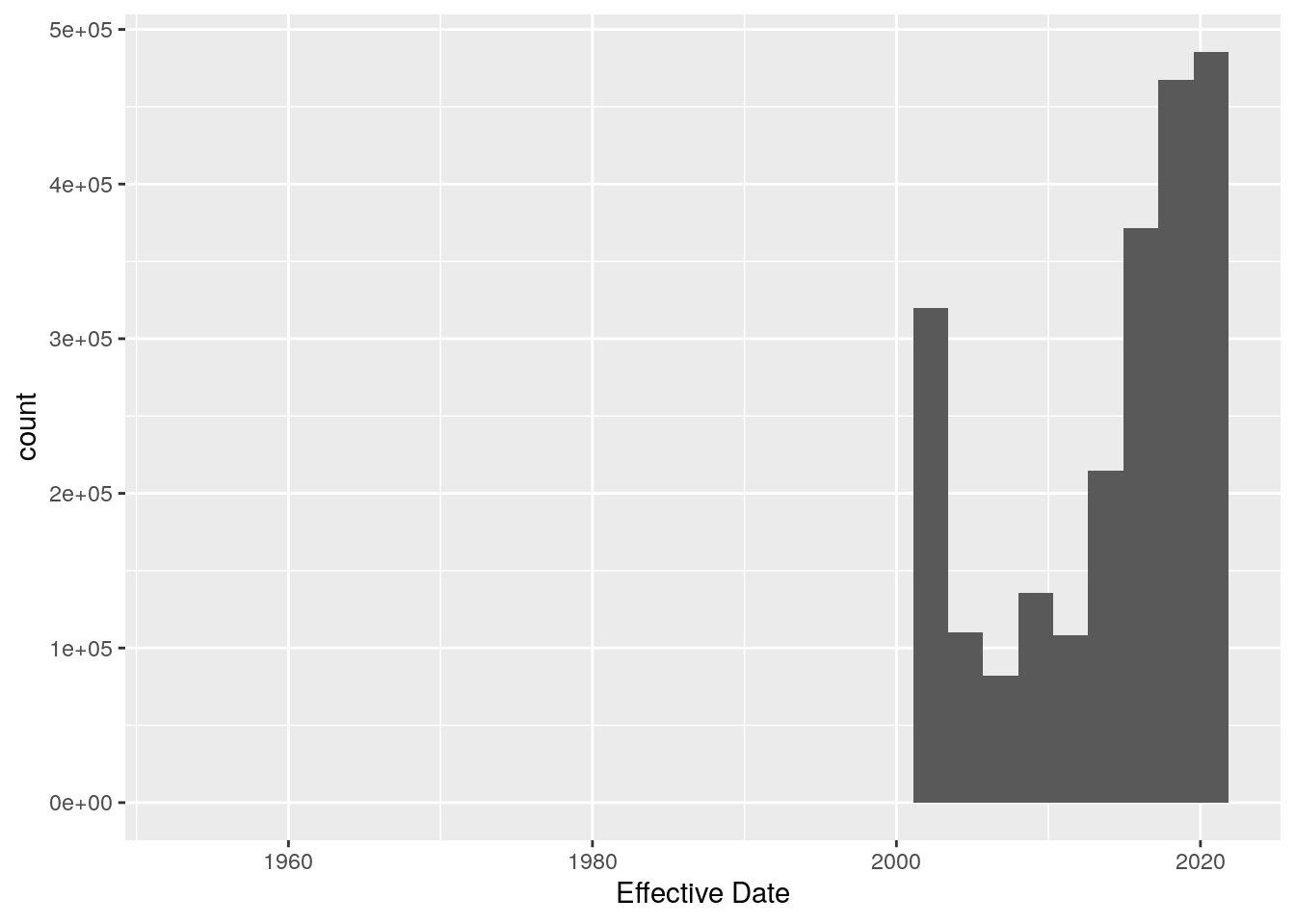
Registered <- Registered %>%
  filter(Status=="Active") %>%
  mutate(`Effective Date`=mdy(`Effective Date`)) %>%
  filter(!is.na(`Effective Date`)) %>%
  mutate(NewVoter=if_else(`Effective Date`>=ymd("2020-01-01"), "NewVoter", "OldVoter")) %>%
  group_by(NewVoter, Zip) %>%
    summarise(Registered=n()) %>%
  ungroup()

Registered <- Registered %>%
  pivot_wider(id_cols=Zip, names_from=NewVoter, values_from=Registered)

###########   ancillary data
path <- "/home/ajackson/Dropbox/Rprojects/Datasets/"

#   SF file of zipcode outlines and areas

Zip_outlines <- readRDS(paste0(path, "ZipCodes_sf.rds"))
Zip_outlines <-  sf::st_as_sf(Zip_outlines) # fix problem due to update to dplyr
#   Census data for 2016

Zip_census16 <- readRDS(paste0(path, "TexasZipcode_16.rds"))
Zip_census16 <- Zip_census16 %>%
  mutate(ZCTA=as.character(ZCTA))

Zip_census16 <- Zip_census16 %>%
  mutate(Race=case_when(
    White/(Pop)>0.5    ~ "White",
    Black/(Pop)>0.5    ~ "Black",
    Hispanic/(Pop)>0.5 ~ "Hispanic",
    TRUE               ~ "Mixed"
    )
  )


#   Median family income and number of families
Income <- readRDS("/home/ajackson/Dropbox/Rprojects/Datasets/IncomeByZip.rds")

#   Many vs 2 generational households
House <- readRDS("/home/ajackson/Dropbox/Rprojects/Datasets/HouseholdByZip.rds")

#   Blueness

Blueness <- readRDS(paste0(path,"HarrisBlueness.rds"))

knitr::opts_chunk$set(warning=FALSE, message=FALSE)
Initial look
First off, let’s explore the data for issues, and for ideas about what might be interesting.
VotesByZip <- VotesByZipDate %>%
  group_by(Zip) %>%
    summarise(Votes=sum(Votes)) %>%
  ungroup()

ByZip <- Zip_census16 %>%
  rename(Zip=ZCTA) %>%
  left_join(VotesByZip,.)

ByZip <- Registered %>%
  left_join(ByZip,.)

ByZip <- Income %>%
  rename(Zip=ZCTA) %>%
  left_join(ByZip,.)

ByZip <- Blueness %>%
  rename(Zip=ZCTA) %>%
  left_join(ByZip,.)

ByZip %>%
  mutate(VotesPct=100*Votes/(NewVoter+OldVoter)) %>%
  filter(Votes>100) %>%
  ggplot(aes(x=VotesPct))+
  geom_histogram()+
  theme(legend.position = "none")+
  labs(x="% Registered Voters", y="Number of Zipcodes",
       title=paste("Percent of Registered Voters Voted by Zipcode",
       today()))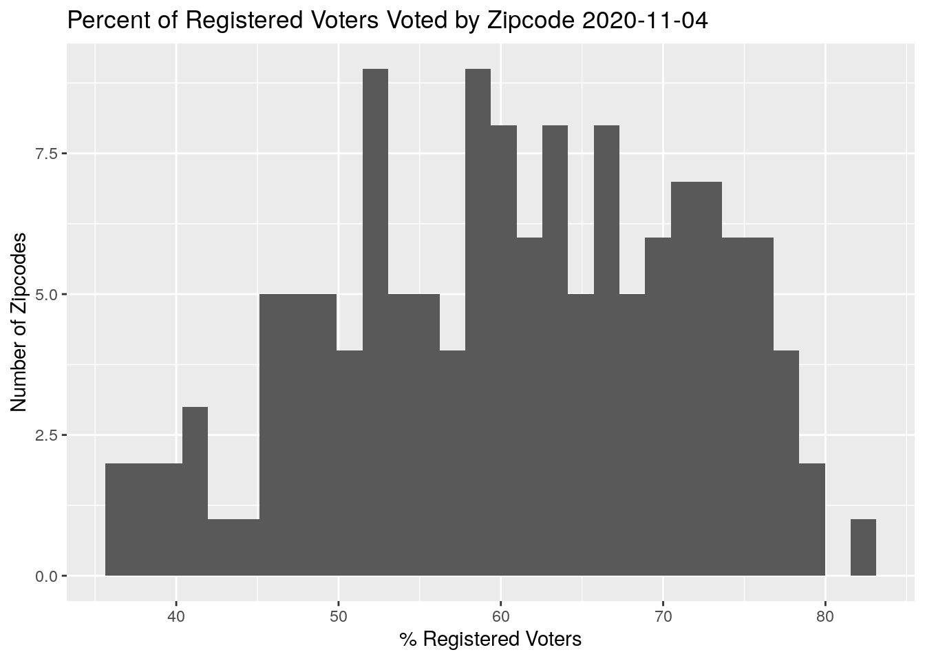
okay let’s have fun
#   Distributions of new and old voters

ByZip %>%
  mutate(Total=NewVoter+OldVoter) %>%
  mutate(NewVoter=100*NewVoter/(Total)) %>%
  mutate(OldVoter=100*OldVoter/(Total)) %>%
  select(Zip, NewVoter, OldVoter) %>%
  pivot_longer(!Zip, names_to="Voter", values_to="Number" ) %>%
  ggplot(aes(x=Number)) +
  geom_density(aes(color=Voter))+
  geom_histogram(aes(color=Voter))+
  labs(x="% of Registered Voters", y="Number of Zip codes",
       title="Proportion of voters new since January 2020")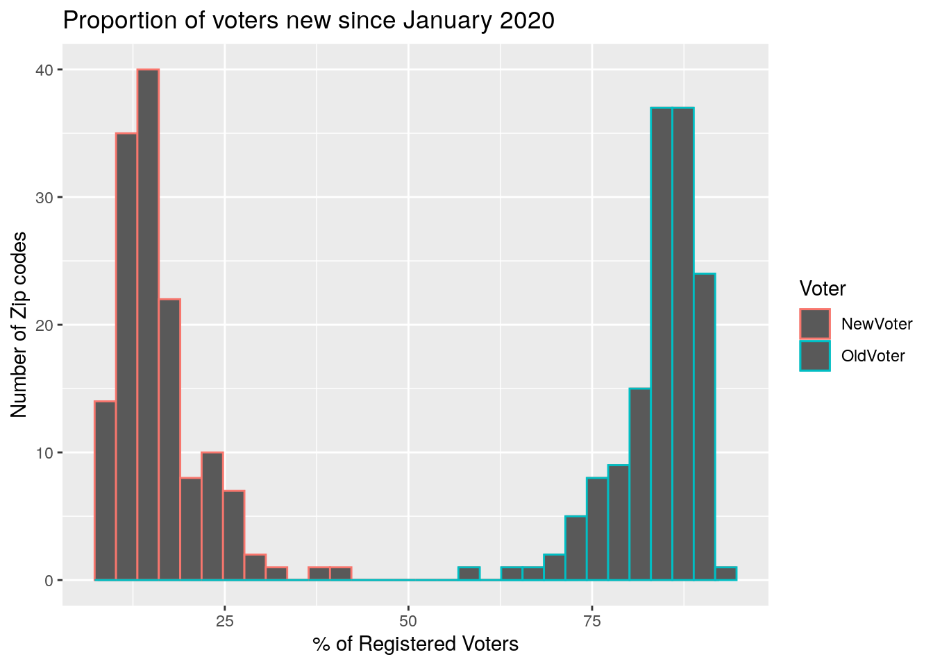
#   New vs blueness

ByZip %>%
  mutate(Total=NewVoter+OldVoter) %>%
  mutate(NewVoter=100*NewVoter/(Total)) %>%
  mutate(OldVoter=100*OldVoter/(Total)) %>%
  select(Zip, NewVoter, OldVoter, blueness) %>%
  ggplot(aes(x=blueness, y=NewVoter)) +
  geom_point()+
  labs(x="% Voted for Hillary Clinton", y="% Registered Voters that are New",
       title="Blueness of Zipcode vs. % New Registered Voters")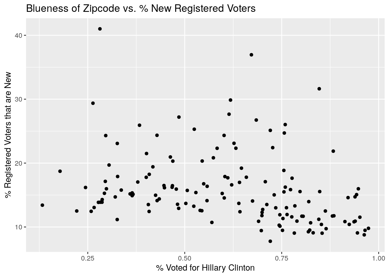
ByZip %>%
  select(Zip, NewVoter, OldVoter, blueness) %>%
  ggplot(aes(x=blueness, y=NewVoter)) +
  geom_point()+
  labs(x="% Voted for Hillary Clinton", y="Number Registered Voters that are New",
       title="Blueness of Zipcode vs. Number of New Registered Voters")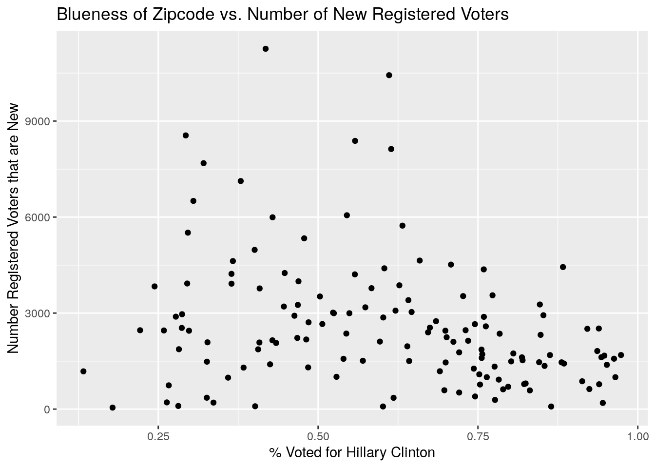
group.colors <- c(Rep = "red", Dem = "blue")
ByZip %>%
  select(Zip, NewVoter, OldVoter, blueness) %>%
  mutate(Dem=NewVoter*blueness,
         Rep=NewVoter*(1-blueness)) %>%
  select(Zip, Rep, Dem) %>%
  pivot_longer(!Zip, names_to="Party", values_to="Number" ) %>%
  ggplot(aes(x=Number)) +
  geom_histogram(aes(fill=Party))+
  scale_fill_manual(values=group.colors)+
  labs(x="Number of New Registered Voters", y="Number of Zip codes",
       title="Proportion of voters new since January 2020")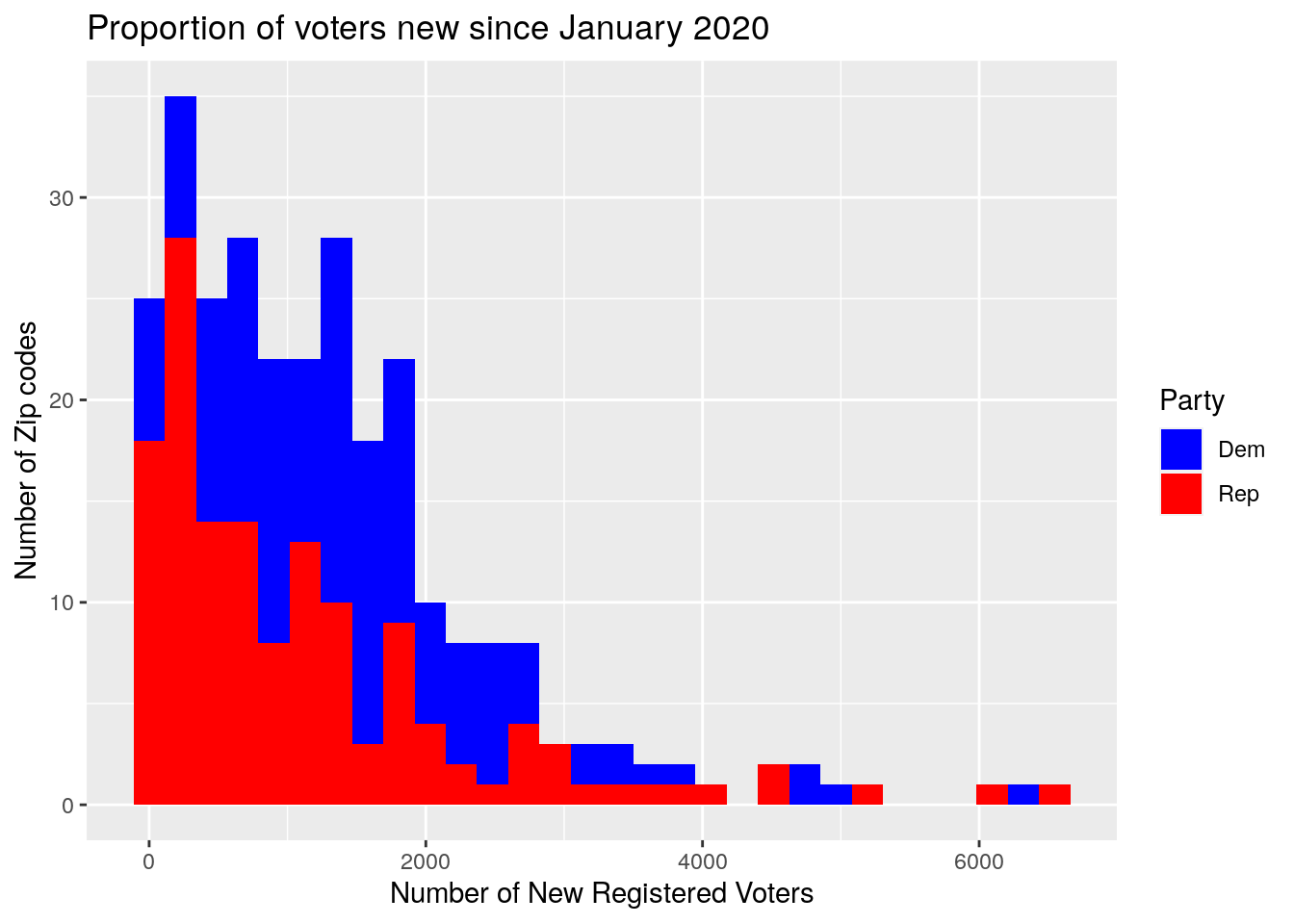
#   % voted vs blueness

ByZip %>%
  select(Zip, Votes, NewVoter, OldVoter, blueness) %>%
  mutate(Pct_Voted=100*Votes/(NewVoter+OldVoter)) %>%
  mutate(blueness=round(blueness*20, 0)/20) %>%
  group_by(blueness) %>%
    summarise(Pct_Voted=100*sum(Votes)/(sum(NewVoter)+sum(OldVoter))) %>%
  ungroup() %>%
  ggplot(aes(x=blueness, y=Pct_Voted)) +
  geom_histogram(stat="identity")+
  labs(x="Percent zipcode voted for Clinton", y="Percent of Registered Voters",
       title="Percent Registered Voters who have Voted vs. Blueness")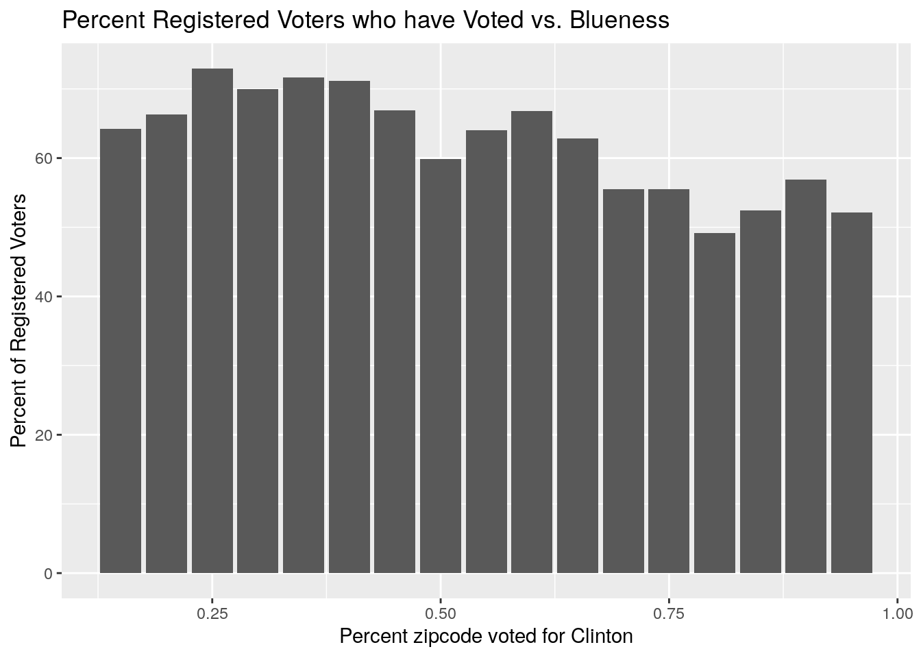
#   % voted vs median age

ByZip %>%
  select(Zip, Votes, NewVoter, OldVoter, MedianAge) %>%
  mutate(Pct_Voted=100*Votes/(NewVoter+OldVoter)) %>%
  mutate(MedianAge=as.numeric((MedianAge))) %>%
  ggplot(aes(x=MedianAge, y=Pct_Voted)) +
  geom_point() +
  geom_smooth(method="lm") +
  labs(x="Median Age", y="Percent of Registered Voters",
       title="Percent Reg Voters who have Voted vs. Median Age in Zipcode")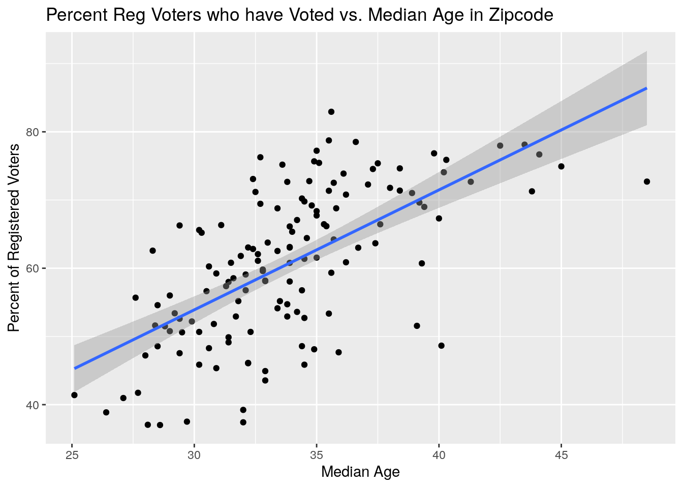
#   % voted vs median income

ByZip %>%
  select(Zip, Votes, NewVoter, OldVoter, Med_Income) %>%
  mutate(Pct_Voted=100*Votes/(NewVoter+OldVoter)) %>%
  ggplot(aes(x=Med_Income, y=Pct_Voted)) +
  geom_point() +
  geom_smooth(method="lm") +
  labs(x="Median Income", y="Percent of Registered Voters",
       title="Percent Reg Voters who have Voted vs. Median Income in Zipcode")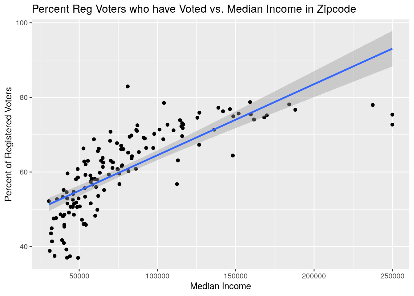
#   % voted vs % black

ByZip %>%
  select(Zip, Votes, NewVoter, OldVoter, Black, Pop) %>%
  mutate(Pct_Voted=100*Votes/(NewVoter+OldVoter),
         Pct_Black=100*Black/Pop) %>%
  ggplot(aes(x=Pct_Black, y=Pct_Voted)) +
  geom_point() +
  geom_smooth(method="lm") +
  labs(x="Percent Black", y="Percent of Registered Voters",
       title="Percent Reg Voters who have Voted vs. Percent Black in Zipcode")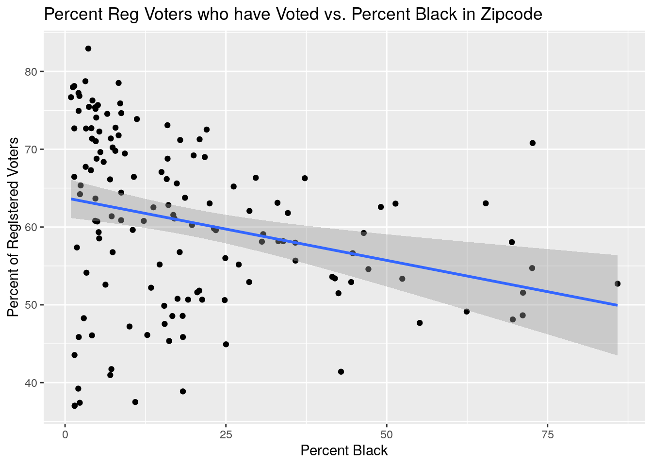
#   % voted vs % hispanic

ByZip %>%
  select(Zip, Votes, NewVoter, OldVoter, Hispanic, Pop) %>%
  mutate(Pct_Voted=100*Votes/(NewVoter+OldVoter),
         Pct_Hispanic=100*Hispanic/Pop) %>%
  ggplot(aes(x=Pct_Hispanic, y=Pct_Voted)) +
  geom_point() +
  geom_smooth(method="lm") +
  labs(x="Percent Hispanic", y="Percent of Registered Voters",
       title="Percent Reg Voters who have Voted vs. Percent Hispanic in Zipcode")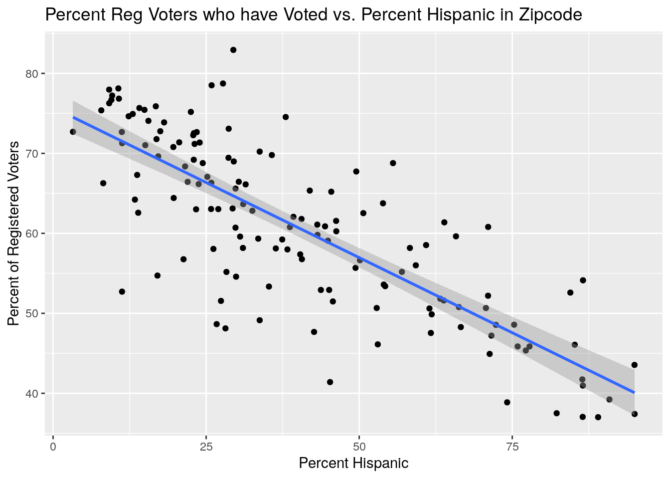
#   % voted vs Age 20-34 %

ByZip %>%
  select(Zip, Votes, NewVoter, OldVoter, Age25to34, Pop) %>%
  mutate(Pct_Voted=100*Votes/(NewVoter+OldVoter),
         Pct_Age25to34=100*Age25to34/Pop) %>%
  ggplot(aes(x=Pct_Age25to34, y=Pct_Voted)) +
  geom_point() +
  geom_smooth(method="lm") +
  labs(x="Percent Age25 to 34", y="Percent of Registered Voters",
       title="Pct Reg Voters who have Voted vs. Pct Age25 to 34 in Zipcode")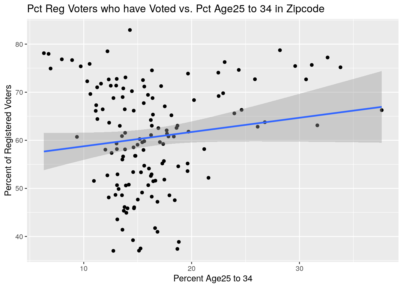
#   # by party per time

VotesByZipDate %>%
  left_join(., Blueness, by=c("Zip"="ZCTA")) %>%
  left_join(., Registered) %>%
  select(Date, Zip, Votes, blueness, Ballot_Type, NewVoter, OldVoter) %>%
  group_by(Ballot_Type, Date) %>%
    summarise(Pct_Voted=100*sum(Votes, na.rm=TRUE)/
                (sum(NewVoter, na.rm = TRUE)+sum(OldVoter, na.rm = TRUE))) %>%
  ungroup() %>%
  group_by(Ballot_Type) %>%
    mutate(Cum_Pct_Voted=cumsum(Pct_Voted)) %>%
  ungroup() %>%
  ggplot(aes(x=Date, y=Cum_Pct_Voted, color=Ballot_Type)) +
  geom_line() +
  geom_point() +
  labs(x="Date", y="Cumulative Percent of Registered Voters",
       title="Percent Registered Voters who have Voted vs. Date")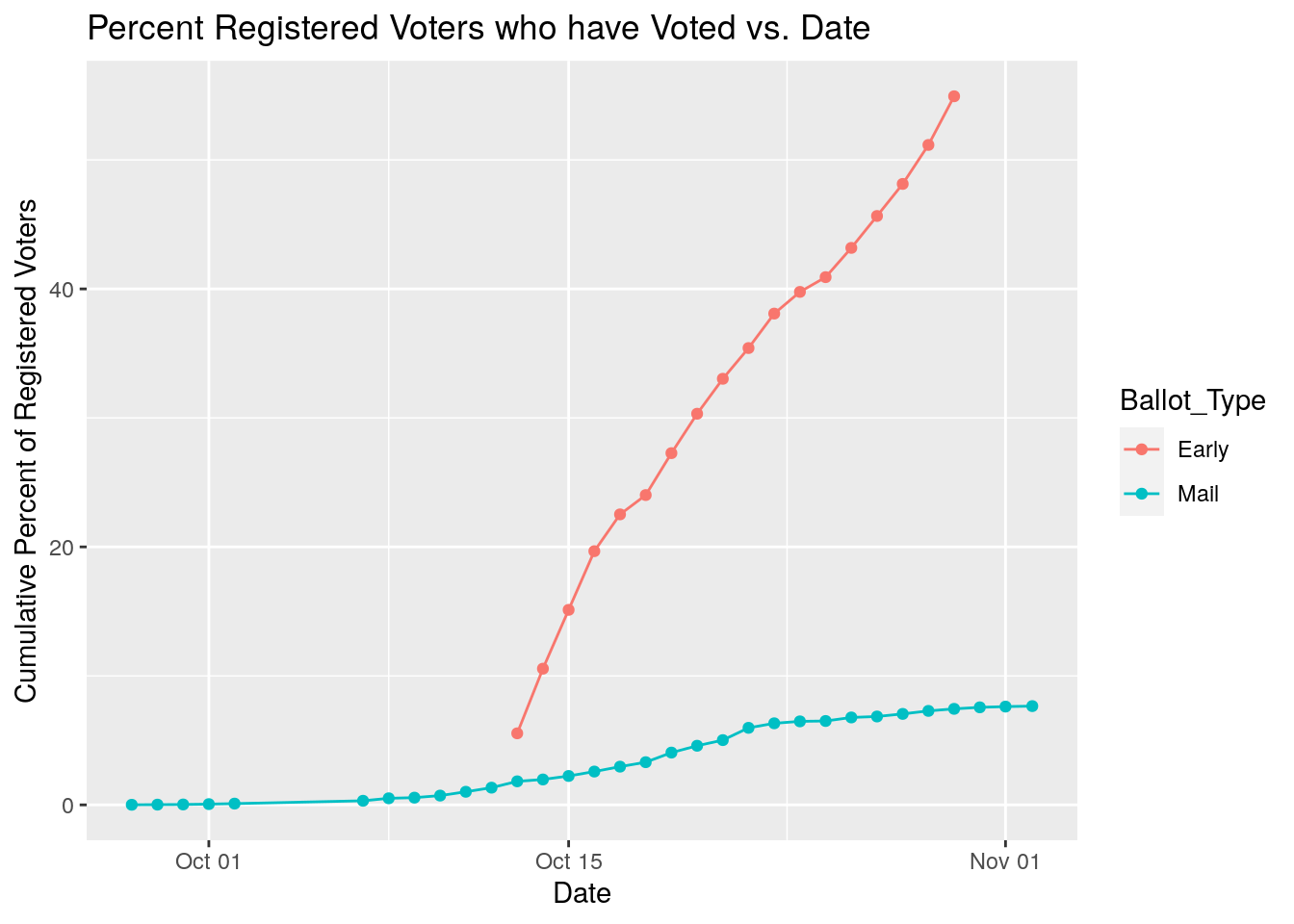
Map
MapData <- ByZip %>%
mutate(Pct_Voted=100*Votes/(NewVoter+OldVoter)) %>%
select(Zip, Pct_Voted)
MapData <- left_join(MapData, Zip_outlines, by=c("Zip"="Zip_Code"))
MapData <- sf::st_as_sf(MapData)
# percent voted by zipcode
kmeans_loc <- c(1+which(diff(kmeans(sort(MapData$Pct_Voted), 5)[["cluster"]])!=0))
kmeans_bins <- signif(c(0,
sort(MapData$Pct_Voted)[kmeans_loc],
max(MapData$Pct_Voted, na.rm=TRUE)),3)
pal <- leaflet::colorBin(palette = heat.colors(5),
bins = 4,
pretty = TRUE,
na.color = "transparent",
domain = MapData$Pct_Voted,
alpha = FALSE,
right = FALSE)
leaflet::leaflet(MapData) %>%
leaflet::setView(lng = -95.3103, lat = 29.7752, zoom = 8 ) %>%
leaflet::addTiles() %>%
leaflet::addPolygons(data = MapData,
weight = 1,
stroke=TRUE,
smoothFactor = 0.2,
fillOpacity = 0.7,
fillColor = ~pal(MapData$Pct_Voted)) %>%
leaflet::addLegend("bottomleft", pal = pal,
values = MapData$Pct_Voted,
labels= as.character(seq(Range[1], Range[2], length.out = 5)),
labFormat = function(type, cuts, p) {
n = length(cuts)
paste0(signif(cuts[-n],2), " – ", signif(cuts[-1],2))
},
title = "Percent Voted per zipcode",
opacity = 1
)and more plots
# Break data into white, hispanic, black majority and mixed classes.
# Plot each group against time.

VotesByZipDate %>%
  left_join(., Zip_census16, by=c("Zip"="ZCTA")) %>%
  left_join(., Registered) %>%
  select(Date, Zip, Votes, Race, NewVoter, OldVoter) %>%
  group_by(Race, Date) %>%
    summarise(Pct_Voted=100*sum(Votes, na.rm=TRUE)/
                (sum(NewVoter, na.rm = TRUE)+sum(OldVoter, na.rm = TRUE))) %>%
  ungroup() %>%
  filter(!is.infinite(Pct_Voted)) %>%
  group_by(Race) %>%
    mutate(Cum_Pct_Voted=cumsum(Pct_Voted)) %>%
  ungroup() %>%
  ggplot(aes(x=Date, y=Cum_Pct_Voted, color=Race)) +
  geom_line() +
  geom_point() +
  labs(x="Date", y="Cumulative Percent of Registered Voters",
       title="Percent Registered Voters who have Voted vs. Date")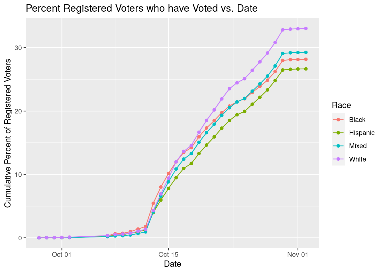
# Do similar with blueness - 4-5 bins of blueness and plot against time.

VotesByZipDate %>%
  left_join(., Blueness, by=c("Zip"="ZCTA")) %>%
  left_join(., Registered) %>%
  select(Date, Zip, Votes, blueness, NewVoter, OldVoter) %>%
  mutate(Blue_Quartile=ntile(blueness, 4)) %>%
  group_by(Blue_Quartile, Date) %>%
    summarise(Pct_Voted=100*sum(Votes, na.rm=TRUE)/
                (sum(NewVoter, na.rm = TRUE)+sum(OldVoter, na.rm = TRUE))) %>%
  ungroup() %>%
  filter(!is.infinite(Pct_Voted)) %>%
  group_by(Blue_Quartile) %>%
    mutate(Cum_Pct_Voted=cumsum(Pct_Voted)) %>%
  ungroup() %>%
  ggplot(aes(x=Date, y=Cum_Pct_Voted, group=Blue_Quartile,
             color=Blue_Quartile)) +
  geom_line() +
  geom_point() +
  labs(x="Date", y="Cumulative Percent of Registered Voters",
       title="Percent Registered Voters who have Voted vs. Date")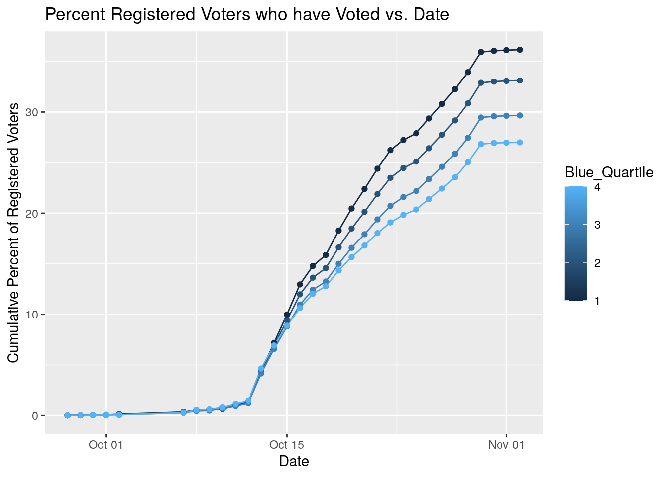
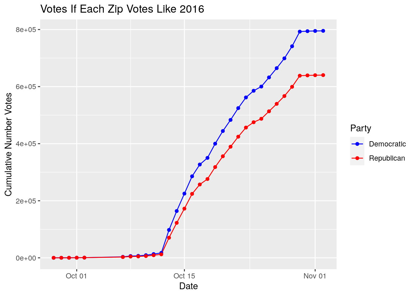
# crossplot pct voted against % covid

# multiply blueness by # voted to estimate R vs Dem actual votes

VotesByZipDate %>%
  left_join(., Blueness, by=c("Zip"="ZCTA")) %>%
  left_join(., Registered) %>%
  select(Date, Zip, Votes, blueness, NewVoter, OldVoter) %>%
  mutate(Republican=Votes*(1-blueness),
         Democratic=Votes*(blueness)) %>%
  select(Date, Democratic, Republican) %>%
  pivot_longer(!Date, names_to="Party", values_to="Votes") %>%
  #   Collapse zipcodes
  group_by(Date, Party) %>%
    summarise(Votes=sum(Votes, na.rm = TRUE)) %>%
  ungroup() %>%
  arrange(Date) %>%
  group_by(Party) %>%
    mutate(Cum_Votes=cumsum(Votes)) %>%
  ungroup() %>%
  ggplot(aes(x=Date, y=Cum_Votes, group=Party,
             color=Party)) +
  geom_line() +
  geom_point() +
  scale_color_manual(values=c(Democratic="blue", Republican="red"))+
  labs(x="Date", y="Cumulative Number Votes",
       title="Votes If Each Zip Votes Like 2016")