Harris County Appraisal District data
Harris County Appraisal District data
Let’s start exploring the data. We’ll look at all these exempt properties.
#   This takes us from 1.4 million to 74,000 records

Dx <- df %>%
  filter(str_detect(state_class, "^X"))

Dx %>%
  ggplot(aes(x=state_class)) +
  geom_histogram(stat="count")+
  labs(x="Exempt code",
       y="Number of Properties",
       title="Number of properties in each exempt class")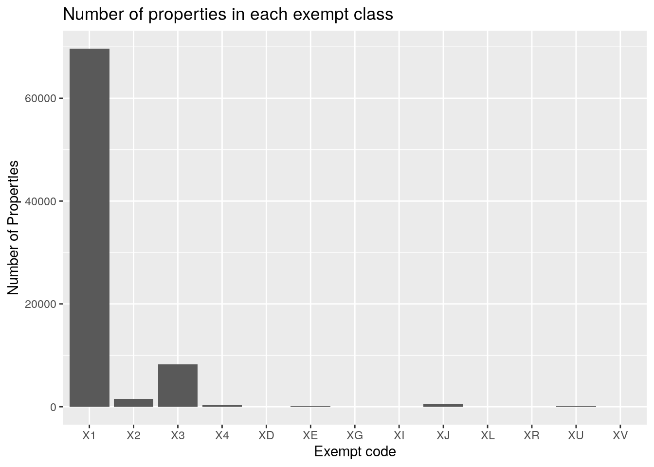
#   Same plot but for total square miles

Dx %>%
  group_by(state_class) %>%
    summarize(area=sum(land_ar, na.rm=TRUE)*3.58701e-8) %>%
  ggplot(aes(x=state_class)) +
  geom_col(aes(y=area))+
  labs(x="Exempt code",
       y="Square Miles",
       title="Area of properties in each exempt class")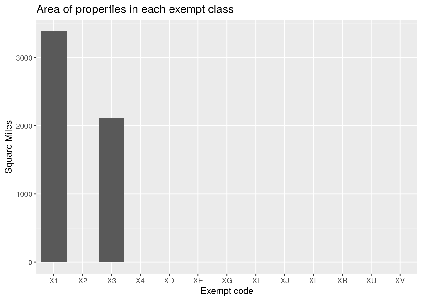
#   Same plot but for total Market Value

Dx %>%
  group_by(state_class) %>%
    summarize(area=sum(tot_mkt_val, na.rm=TRUE)) %>%
  ggplot(aes(x=state_class)) +
  geom_col(aes(y=area))+
  labs(x="Exempt code",
       y="Market Value in Dollars",
       title="Market Value of properties in each exempt class")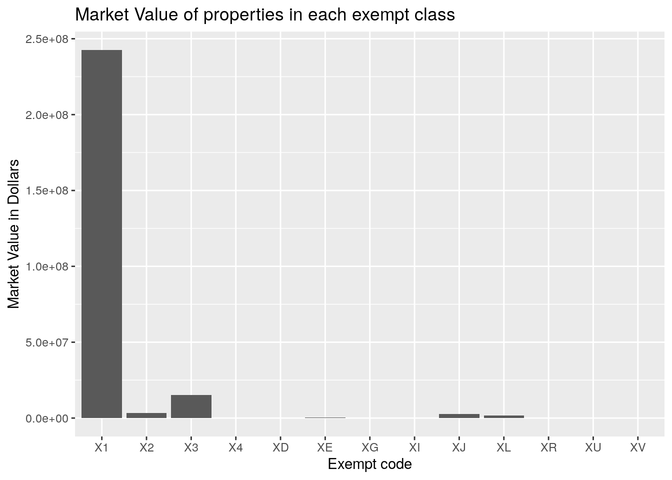
Dx %>%
filter(state_class=="X1" |
state_class=="X2" |
state_class=="X3") %>%
mutate(state_class=case_when(state_class=="X1" ~ "Government",
state_class=="X2" ~ "Charitable",
state_class=="X3" ~ "Religious",
TRUE ~ "Error")) %>%
ggplot(aes(x=tot_mkt_val )) +
geom_histogram() +
scale_y_log10() +
facet_wrap(vars(state_class), scales="free")+
labs(y="Count",
x="Market Value in Dollars",
title="Market Value of properties in each exempt class")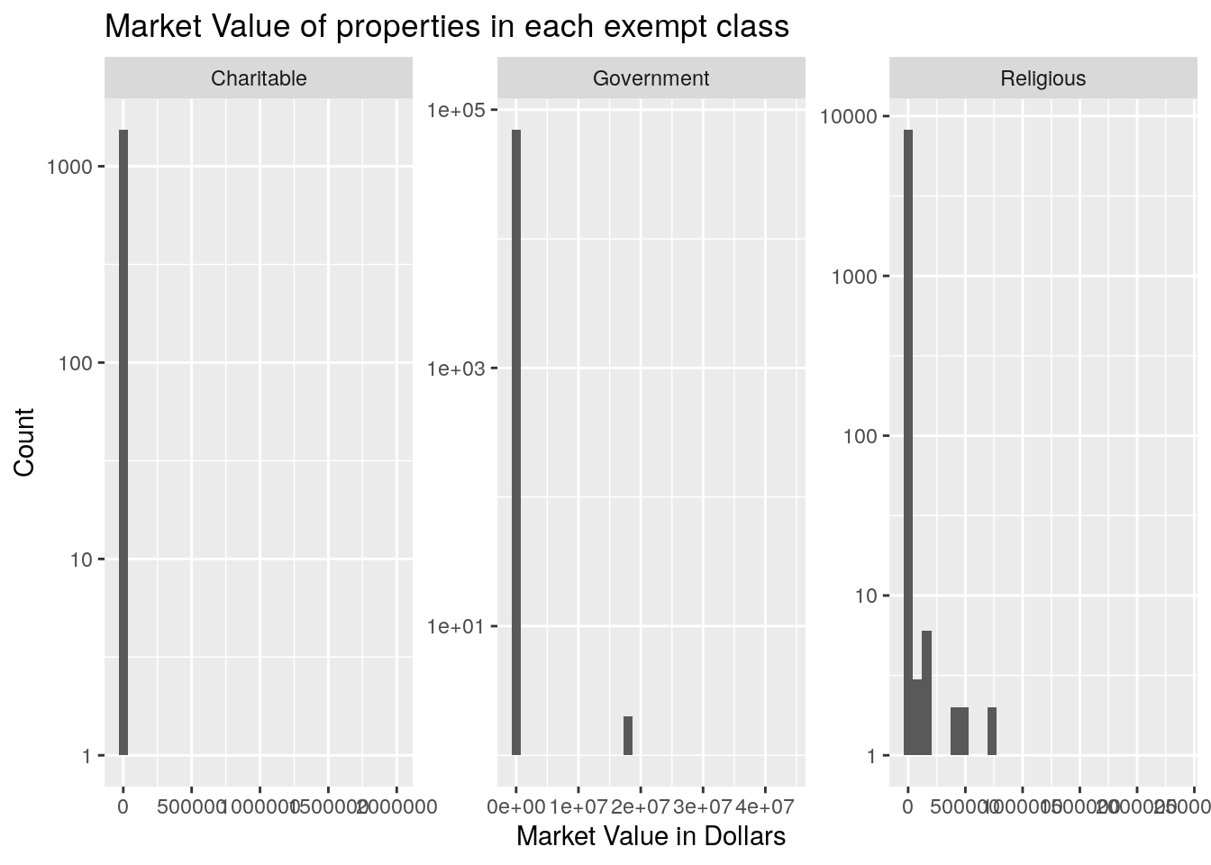 So the code X1 means “Other Exempt (Government)”, and X3 means “Other Exempt
(Religious)”. Apparently the number of square miles for exempt government
property is about equal to that of religious property, but the value of the
religious property is much less. But to be fair, much of the government
property has a value of zero. Actually much of the exempt property has a “value”
of zero. It is a little curious that it isn’t all zero, but maybe the tracts
with value used to be non-exempt and that old value has been carried forward.
So the code X1 means “Other Exempt (Government)”, and X3 means “Other Exempt
(Religious)”. Apparently the number of square miles for exempt government
property is about equal to that of religious property, but the value of the
religious property is much less. But to be fair, much of the government
property has a value of zero. Actually much of the exempt property has a “value”
of zero. It is a little curious that it isn’t all zero, but maybe the tracts
with value used to be non-exempt and that old value has been carried forward.
Now let’s look at he non-exempt properties. We’ll start with all of them and then drill down a bit.
#   This removes 74,000 records

Dnx <- df %>%
  filter(!str_detect(state_class, "^X")) %>%
  mutate(land_ar_mi=land_ar*3.58701e-8) # convert to square miles

#   Delete records with obviously bad data

Dnx <- Dnx %>%
  filter(land_ar_mi<10)

#   Number of properties in each class

Dnx %>%
  ggplot(aes(x=state_class)) +
  geom_histogram(stat="count")+
  labs(x="Code",
       y="Number of Properties",
       title="Number of properties in each non-exempt class")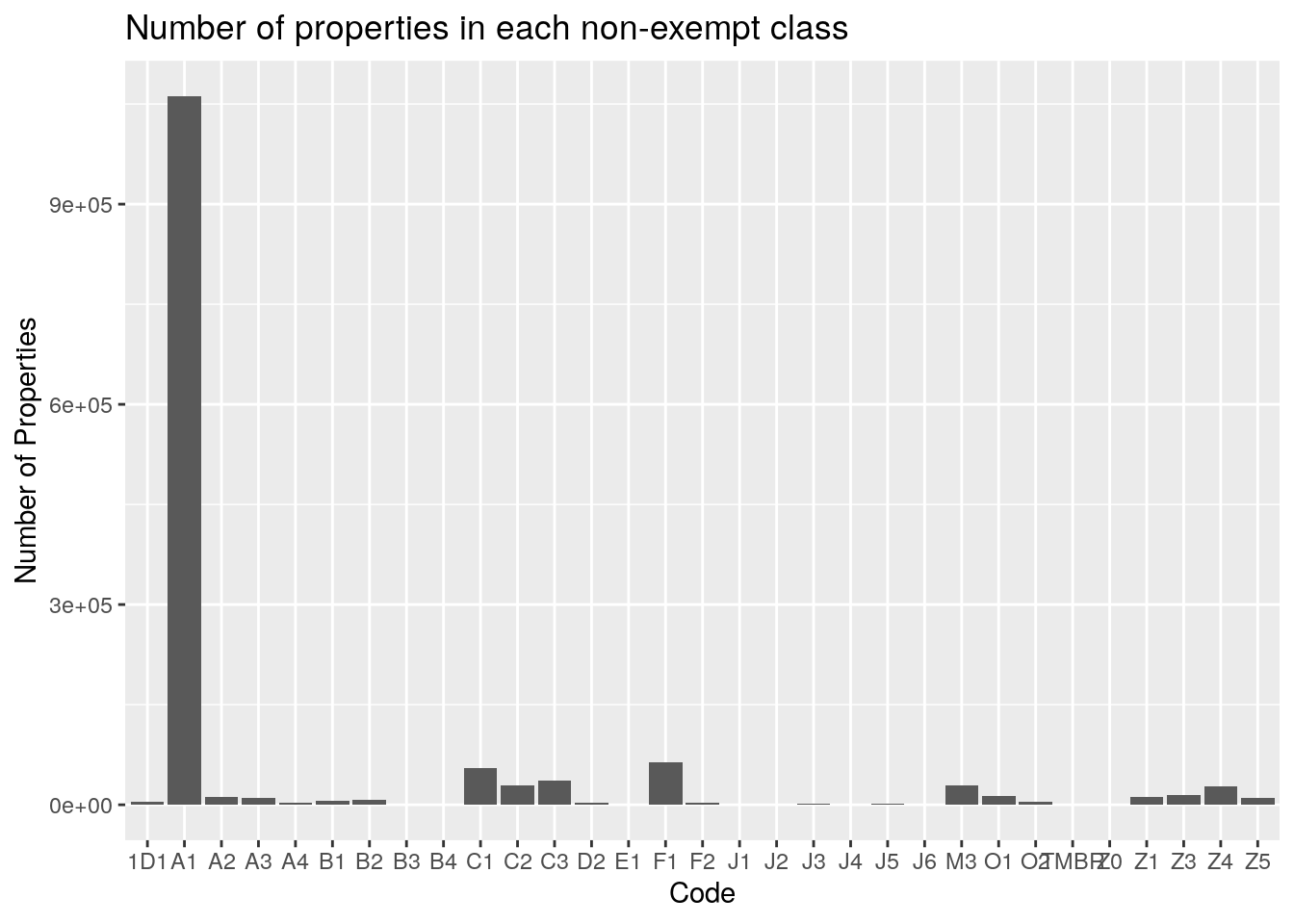
#   Same plot but for total square miles

Dnx %>%
  group_by(state_class) %>%
    #summarize(area=sum(land_ar, na.rm=TRUE)*3.58701e-8) %>%
    summarize(area=sum(land_ar_mi, na.rm=TRUE)) %>%
  ggplot(aes(x=state_class)) +
  geom_col(aes(y=area))+
  labs(x="Code",
       y="Square Miles",
       title="Area of properties in each non-exempt class")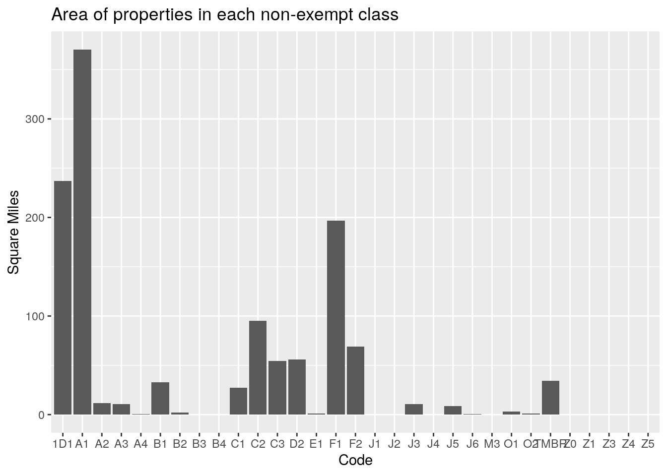
#   Same plot but for total Market Value

Dnx %>%
  group_by(state_class) %>%
    summarize(area=sum(tot_mkt_val, na.rm=TRUE)) %>%
  ggplot(aes(x=state_class)) +
  geom_col(aes(y=area))+
  labs(x="Code",
       y="Market Value in Dollars",
       title="Market Value of properties in each non-exempt class")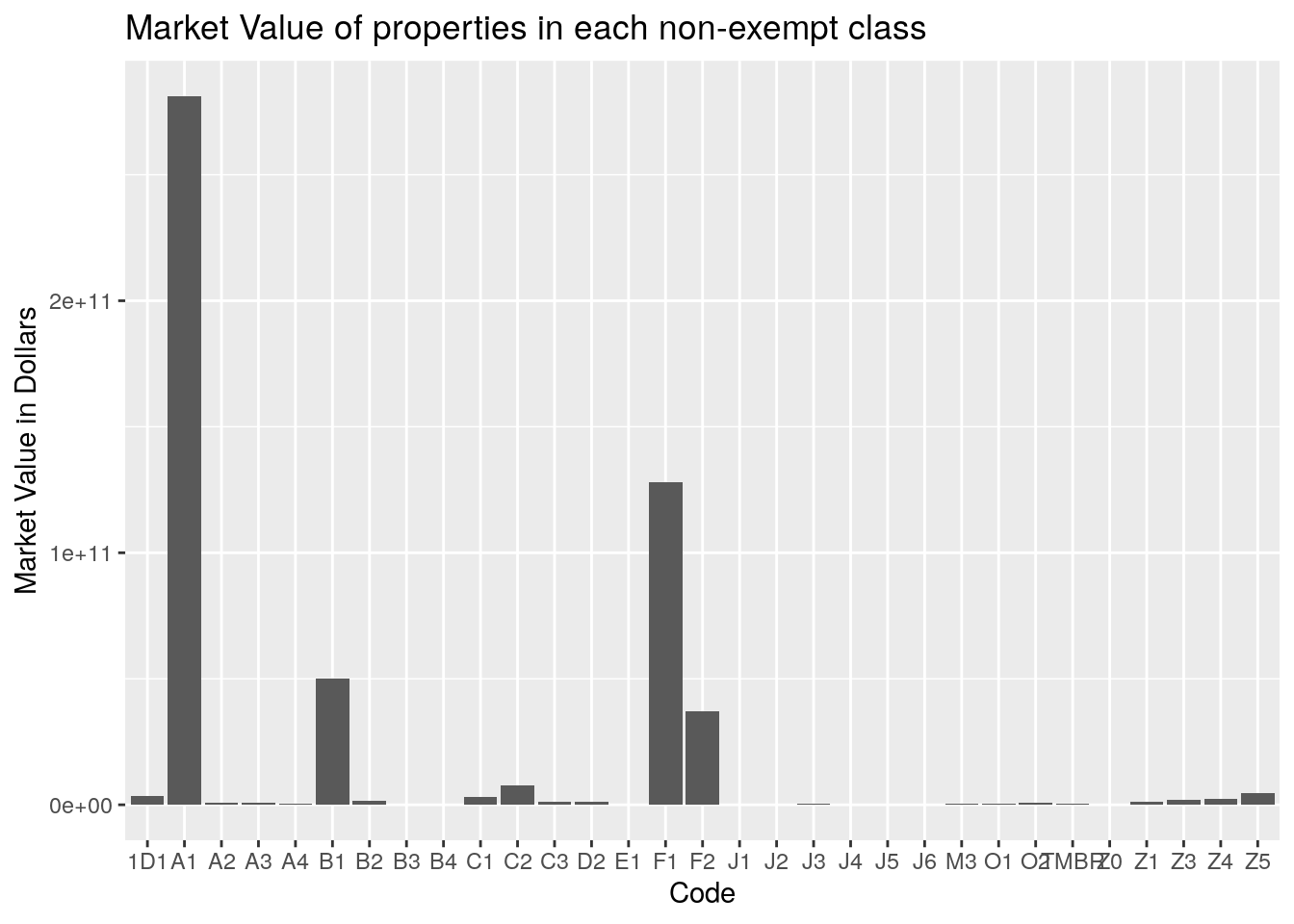
Dnx %>%
  filter(state_class=="A1" |
         state_class=="A2" |
         state_class=="F1" |
         state_class=="F2" |
         state_class=="1D1" |
         state_class=="B1") %>%
  mutate(state_class=case_when(state_class=="A1" ~ "Residential",
                               state_class=="A2" ~ "Mobile Homes",
                               state_class=="B1" ~ "Multi-Family",
                               state_class=="F1" ~ "Commercial",
                               state_class=="F2" ~ "Industrial",
                               state_class=="1D1" ~ "Agricultural",
                               TRUE ~ "Error")) %>%
  ggplot(aes(x=tot_mkt_val )) +
  geom_histogram() +
  scale_y_log10() +
  facet_wrap(vars(state_class), scales="free")+
  labs(y="Count",
       x="Market Value in Dollars",
title="Market Value of properties in each non-exempt class") 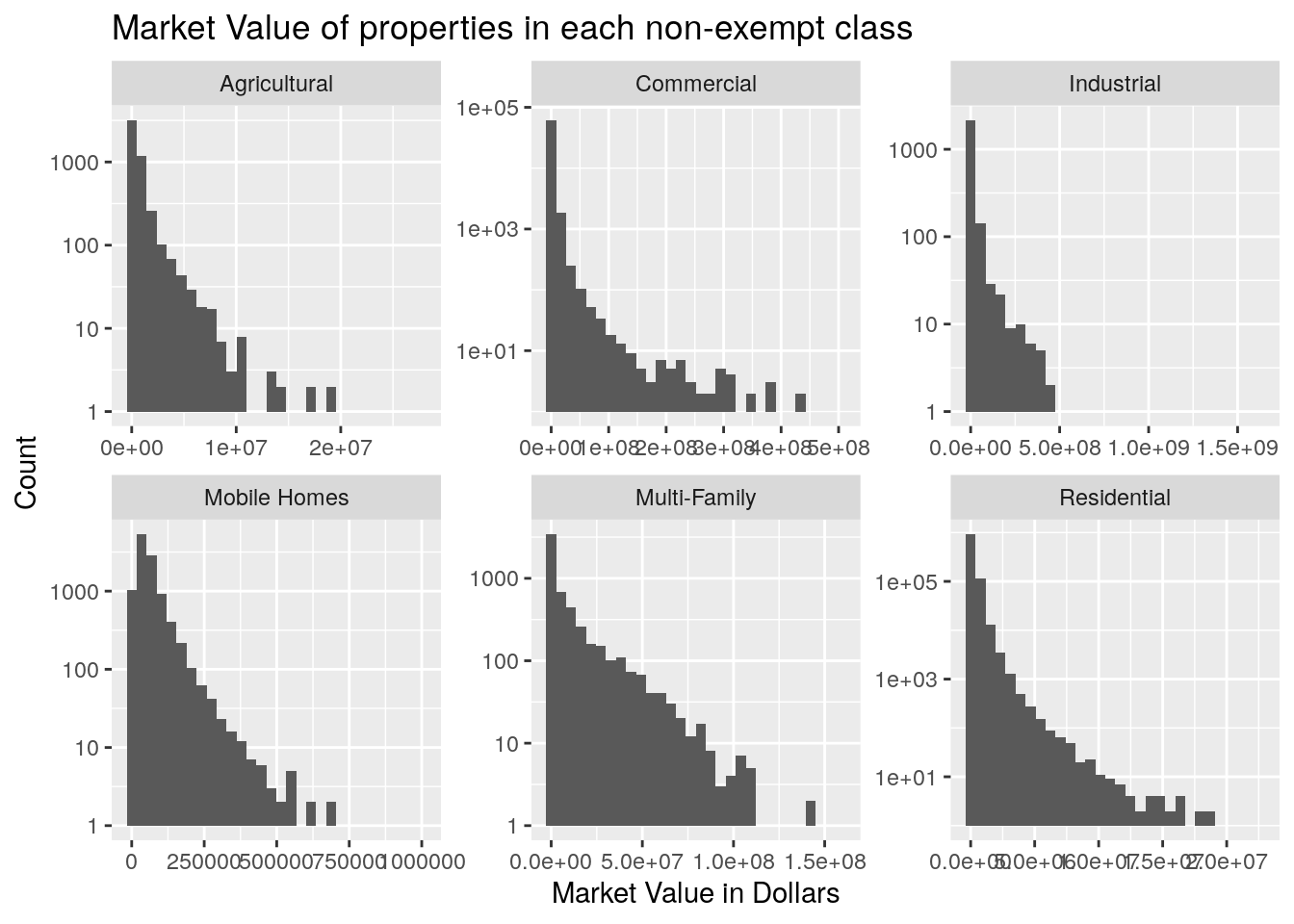
Dnx %>%
  filter(state_class=="A1" |
         state_class=="A2" |
         state_class=="F1" |
         state_class=="F2" |
         state_class=="1D1" |
         state_class=="B1") %>%
  mutate(state_class=case_when(state_class=="A1" ~ "Residential",
                               state_class=="A2" ~ "Mobile Homes",
                               state_class=="B1" ~ "Multi-Family",
                               state_class=="F1" ~ "Commercial",
                               state_class=="F2" ~ "Industrial",
                               state_class=="1D1" ~ "Agricultural",
                               TRUE ~ "Error")) %>%
  ggplot() +
  geom_histogram(aes(x=land_ar_mi)) +
  scale_y_log10() +
  facet_wrap(vars(state_class), scales="free")+
  labs(y="Count",
       x="Land Area (square miles)",
       title="Land Area of properties in each non-exempt class")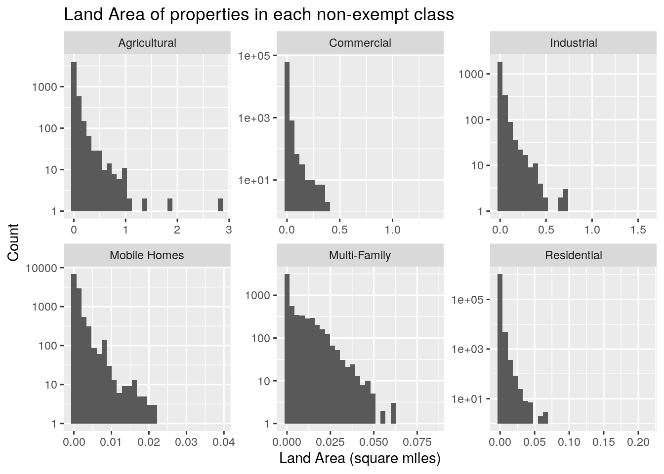
#   Let's build a little table showing how many zero values there are
#   in each class: zeros for area and value

Dnx %>%
  group_by(state_class) %>%
    summarize(across(c("land_ar_mi", "tot_mkt_val"),
                     funs(sum(.==0, na.rm=TRUE))),
                     n=n()) %>%
  mutate(land_pct=land_ar_mi_sum/n,
         value_pct=tot_mkt_val_sum/n) %>%
  select(state_class, land_pct, value_pct) %>%
 gt() %>%
  fmt_percent(columns=c(land_pct, value_pct)) %>%
  cols_label(state_class="Class",
             land_pct="Land Area",
             value_pct="Market Value") %>%
tab_header("Percent of Properties With a Value of Zero")| Percent of Properties With a Value of Zero | ||
|---|---|---|
| Class | Land Area | Market Value |
| 1D1 | 0.02% | 0.00% |
| A1 | 0.85% | 0.00% |
| A2 | 0.21% | 0.00% |
| A3 | 0.99% | 0.00% |
| A4 | 0.00% | 0.00% |
| B1 | 0.07% | 0.00% |
| B2 | 0.17% | 0.00% |
| B3 | 0.19% | 0.00% |
| B4 | 0.00% | 0.00% |
| C1 | 0.61% | 0.00% |
| C2 | 0.11% | 0.00% |
| C3 | 0.81% | 0.00% |
| D2 | 0.43% | 0.00% |
| E1 | 0.21% | 0.00% |
| F1 | 1.01% | 0.00% |
| F2 | 18.50% | 0.00% |
| J1 | 33.87% | 0.00% |
| J2 | 6.25% | 0.00% |
| J3 | 1.68% | 0.00% |
| J4 | 0.66% | 0.00% |
| J5 | 22.73% | 97.90% |
| J6 | 2.78% | 0.00% |
| M3 | 100.00% | 0.00% |
| O1 | 0.00% | 0.00% |
| O2 | 0.05% | 0.00% |
| TMBR | 0.00% | 0.00% |
| Z0 | 99.86% | 0.00% |
| Z1 | 99.64% | 0.00% |
| Z3 | 99.68% | 0.00% |
| Z4 | 99.41% | 0.00% |
| Z5 | 99.53% | 0.00% |
Dnzero <- Dnx %>%
  filter(str_detect(site_addr_1, "^0 "))
Almost all the properties are A1 - single-family residential. Those are also the greatest land area, though 1D1 (Agricultural land) and F1 (Commercial) also come in pretty high. Market value dominated by the big four - single-family residential, commercial, multi-family residential, and industrial. Note that I filtered out all properties with a land area greater than ten square miles. Most categories have a small fraction, less than 1%, of properties with a land area of zero. The exceptions are industrial, utilities (MUDs?), railroads, and mobile homes. Mobile home (M3) owners apparently never own the land their home sits on. Or maybe it no longer counts as a mobile home if they do. The Zx properties are all condos, so there condo owners rarely own the land, the condo association does. For the other categories with less than 1%, I did find a house that is a parsonage, so I assume that the church owns the land and the pastor owns the house itself.
Let us now look at addresses that begin with zero. What is that all about?
I think most of them are where the land is owned by an entity separate from the buildings, and so there is not really a good address. Others are new builds that have not been recorded with an address yet. It pops up the following year.
#   Number of zero address properties

Dnx %>%
  filter(str_detect(site_addr_1, "^0 ")) %>%
  ggplot(aes(x=state_class)) +
  geom_histogram(stat="count")+
  labs(x="Code",
       y="Number of Properties",
       title="Number of properties with an address of zero")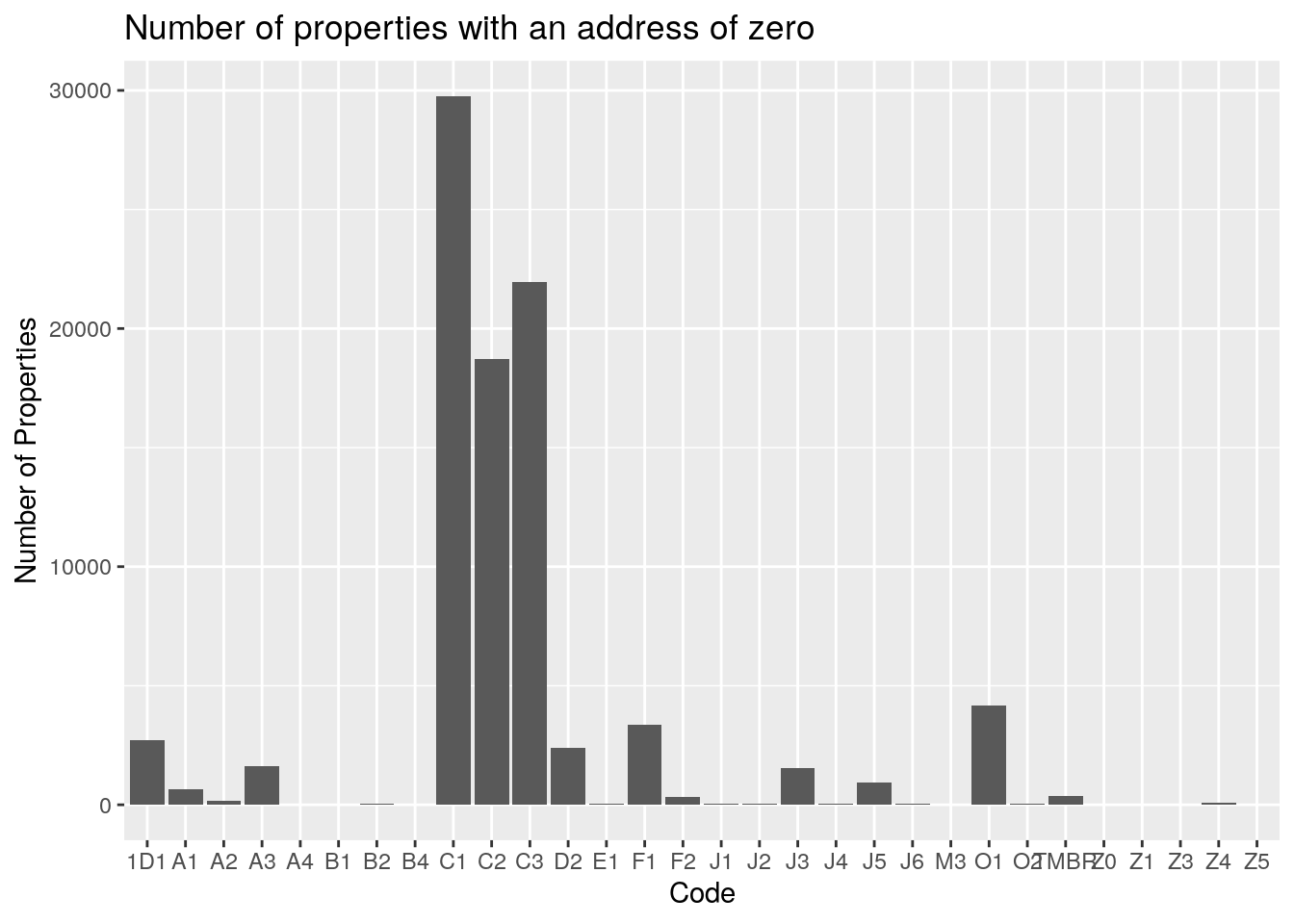
So not surprisingly, most of the properties with an address of zero turn out to be vacant lots (C1, C2, C3) - which largely do not have an address yet.
Analysis
Enough trying to understand the subtlties of the data, let’s do some analysis.
How about the mean and median values of residential real property, land and buildings, by zipcode? But to make comparisons meaningful, let’s normalize all the values by the area, so everything in dollars per square foot.
#   single-family homes

DfMed <- df %>%
  filter(state_class=="A1") %>%
  mutate(land_val=na_if(land_val, 0),
         bld_val=na_if(bld_val, 0)) %>%
  group_by(site_addr_3) %>%
     summarize(mean_land_val=mean(land_val/land_ar, na.rm=TRUE),
               med_land_val=median(land_val/land_ar, na.rm=TRUE),
               mean_bld_val=mean(bld_val/bld_ar, na.rm=TRUE),
               med_bld_val=median(bld_val/bld_ar, na.rm=TRUE)
               ) %>%
  pivot_longer(-site_addr_3,names_to="statistic", values_to="Value")

  DfMed$statistic <- as.factor(DfMed$statistic)
  levels(DfMed$statistic) <- c("Mean Building Value per Sq-Ft",
                               "Mean Land Value per Sq-Ft",
                               "Median Building Value per Sq-Ft",
                               "Median Land Value per Sq-Ft")
  DfMed %>%
  ggplot() +
  geom_histogram(aes(x=Value)) +
  facet_wrap(~statistic, scales="free") +
  labs(y="Number of zip codes",
       x="Value in Dollars per Square-foot",
       title="Mean and Median Land and Building Values by Zipcode")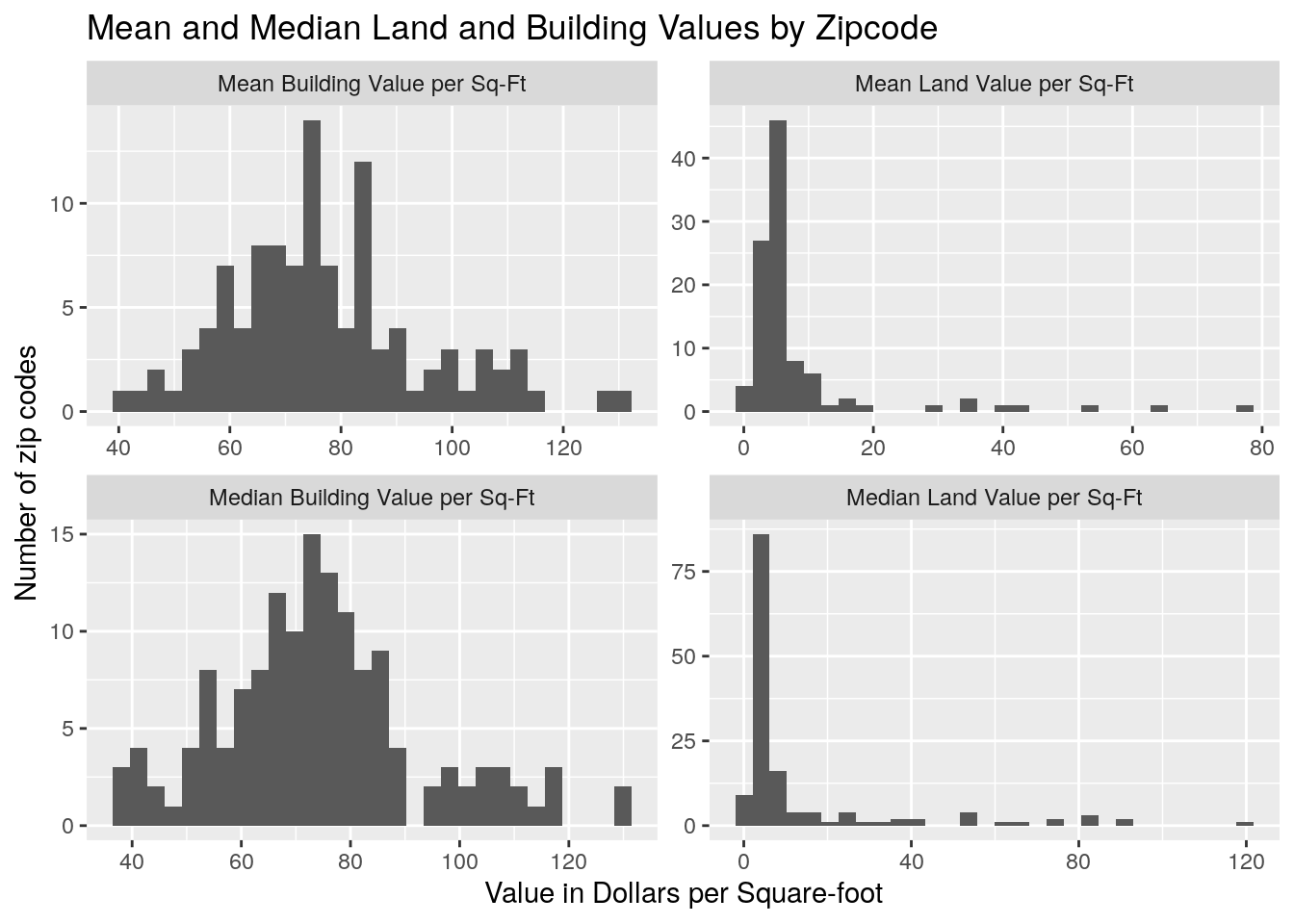
  #   Let's look at the largest and smallest in detail

Df_A1 <- df %>%
  filter(state_class=="A1") %>%
  mutate(land_val=na_if(land_val/land_ar, 0),
         bld_val=na_if(bld_val/bld_ar, 0)) %>%
  select(site_addr_3, bld_val, land_val, acct)

Large_median_land_zips <-
  DfMed %>%
  pivot_wider(names_from = "statistic", values_from = Value) %>%
  filter(`Median Land Value per Sq-Ft` > 20) %>%
  select(site_addr_3)

p_hi_land <- Df_A1 %>%
  filter(site_addr_3 %in% Large_median_land_zips$site_addr_3) %>%
  mutate(Data_subset = "Expensive Land") %>%
  mutate(Value=land_val)

Large_median_bld_zips <-
  DfMed %>%
  pivot_wider(names_from = "statistic", values_from = Value) %>%
  filter(`Median Building Value per Sq-Ft` > 105) %>%
  select(site_addr_3)

p_hi_bld <- Df_A1 %>%
  filter(site_addr_3 %in% Large_median_bld_zips$site_addr_3) %>%
  mutate(Data_subset = "Expensive Buildings") %>%
  mutate(Value=bld_val)

Small_median_land_zips <-
  DfMed %>%
  pivot_wider(names_from = "statistic", values_from = Value) %>%
  filter(`Median Land Value per Sq-Ft` < 2) %>%
  select(site_addr_3)

p_lo_land <- Df_A1 %>%
  filter(site_addr_3 %in% Small_median_land_zips$site_addr_3) %>%
  mutate(Data_subset = "Cheap Land") %>%
  mutate(Value=land_val)

Small_median_bld_zips <-
  DfMed %>%
  pivot_wider(names_from = "statistic", values_from = Value) %>%
  filter(`Median Building Value per Sq-Ft` < 50) %>%
  select(site_addr_3)

p_lo_bld <- Df_A1 %>%
  filter(site_addr_3 %in% Small_median_bld_zips$site_addr_3) %>%
  mutate(Data_subset = "Cheap Buildings") %>%
  mutate(Value=bld_val)

bind_rows(p_hi_land, p_hi_bld, p_lo_land, p_lo_bld) %>%
  ggplot(aes(x=Value)) +
    geom_histogram() +
    facet_wrap(vars(Data_subset), scales="free") +
  labs(y="Number of Properties",
       x="Dollars per square foot",
       title="Properties at ends of the overall distributions",
       subtitle="All properties from zipcodes with high or low values")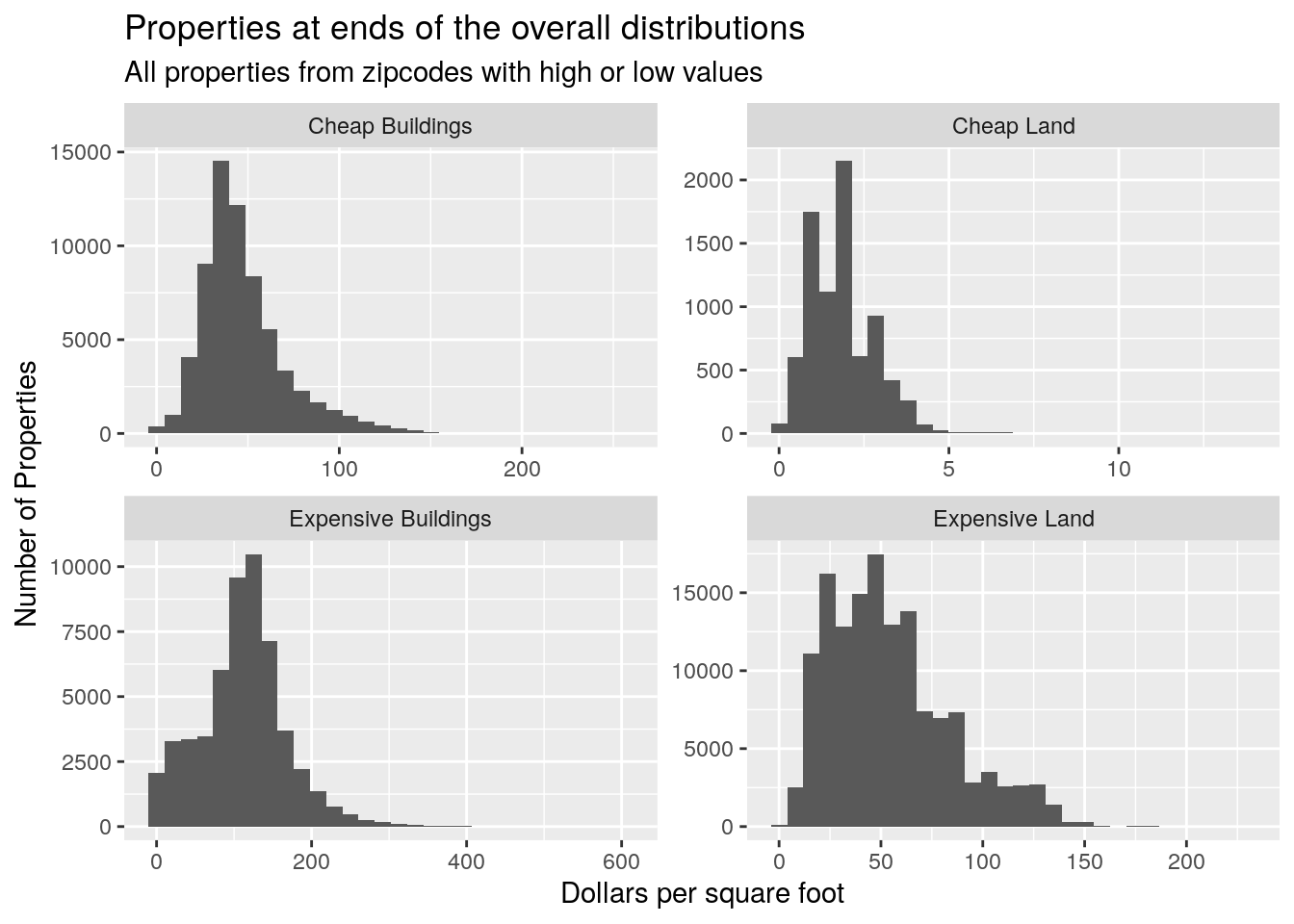
Looks like the median value of residential land is around $5/sq-ft. For residential buildings, there is a large variability, with an average around $75.
In the most expensive zipcodes, the land is really quite pricey, with lots going well above $50/sq-ft, where in the cheap zipcodes, almost nothing goes for more than $5/sq-ft. Residential building values are closer, only a factor of 2 apart.
Now let’s look at one zipcode, 77008, and see what the various proportions are for different residential property types.
Df_Res <- df %>%
  filter(site_addr_3=="77008") %>%
  filter(str_detect(state_class, "^A|B")) %>%
  #   Single family only
 # filter(str_detect(state_class, "^A1")) %>%
  select(acct, yr, state_class, site_addr_1, bld_val, land_val, tot_mkt_val, new_own_dt)

Df_Res %>%
  ggplot(aes(x=state_class)) +
  geom_histogram(stat="count") +
  labs(x="Residential Property Type",
       y="Number of properties",
       title="Distribution of Residential Property Types in Zip Code 77008")
## Warning: Ignoring unknown parameters: binwidth, bins, pad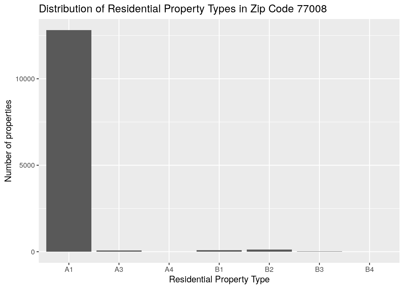
Df_Res <- df %>%
  filter(site_addr_3=="77008") %>%
  filter(str_detect(state_class, "^A|B")) %>%
  #   Single family only
  filter(str_detect(state_class, "^A1")) %>%
  select(acct, yr, state_class, site_addr_1, bld_val, land_val, tot_mkt_val, new_own_dt)
Time for some fun.
Let’s start by looking at one zipcode over time, and develop some interesting plots, which we can then extend to all zipcodes.
#   First do some cleanup

rm(Df_A1, Df_Res, Dnx, Dnzero, Dx, p_hi_bld, p_hi_land, p_lo_bld, p_lo_land)

#   Pull out 77008

df <- readRDS(paste0(DataHCAD, "Values_2020.rds"))
df <- df %>%
  filter(site_addr_3=="77008")
df <- df %>%
  mutate(across(contains(c("_val", "_ar")), make_numeric)) %>%
  mutate(new_own_dt=lubridate::mdy(new_own_dt))

#   Now read in the other files, extract 77008, and then join to df


make_numeric <- function(x){as.numeric(x)}

for (year in "2005":"2019") {

  print(year)

  Df <- readRDS(paste0(DataHCAD, "Values_", year, ".rds"))

  Df <- Df %>%
    filter(site_addr_3=="77008") %>%
    mutate(across(contains(c("_val", "_ar")), make_numeric)) %>%
    mutate(new_own_dt=lubridate::mdy(new_own_dt))

  df <- bind_rows(df, Df)

}
## [1] 2005
## [1] 2006
## [1] 2007
## [1] 2008
## [1] 2009
## [1] 2010
## [1] 2011
## [1] 2012
## [1] 2013
## [1] 2014
## [1] 2015
## [1] 2016
## [1] 2017
## [1] 2018
## [1] 2019# Save in case
saveRDS(df, paste0(DataHCAD, "Data_for_77008.rds"))Let’s see what sort of time dependent stuff is possible
#   Read in

df <- readRDS(paste0(DataHCAD, "Data_for_77008.rds"))

# Mobile homes vs year

df %>%
  filter(state_class=="M3") %>%
  group_by(yr) %>%
  tally() %>%
  #count(yr) %>%
  mutate(yr=as.numeric(yr)) %>%
  ggplot(aes(x=yr, y=n)) +
    geom_point() +
    geom_line() +
    labs(x="Year",
         y="Number of Mobile Homes",
         title="Mobile Homes in 77008",
         subtitle="Data from HCAD Tax Rolls")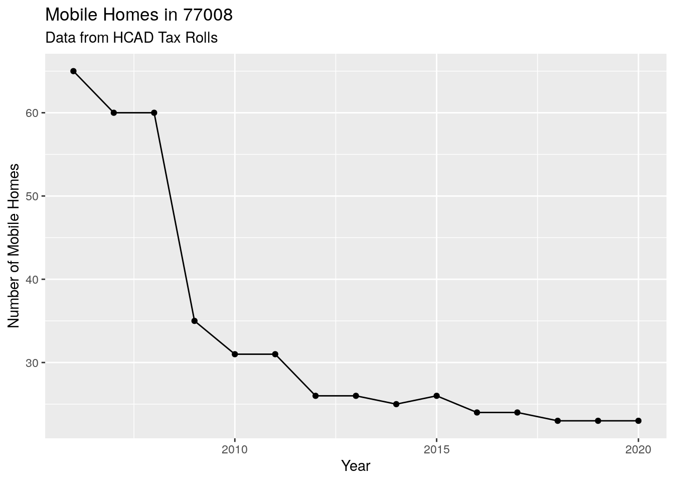
# First let's look for properties that have changed owner since 2005

Changed <- df %>%
  filter(new_own_dt>="2005-01-01")

# Owner changes per year

Owner_changes <- df %>%
  filter(site_addr_3 == "77008") %>%
  select(site_addr_1, new_own_dt) %>%
  unique() %>%
  mutate(year=lubridate::year(new_own_dt)) %>%
  group_by(year) %>%
    tally()

#   Looks like data for 1988 is bogus, so delete if before 1989
#   Also, delete if NA and delete if > 2020

Owner_changes <- Owner_changes %>%
  filter(year>=1989, year<=2020, !is.na(year))

Owner_changes %>%
  ggplot(aes(x=year, y=n)) +
  geom_point() +
  labs(x="Year of Ownership Change",
       y="Number of Properties Changing Ownership",
       title="Ownership Changes in Zipcode 77008")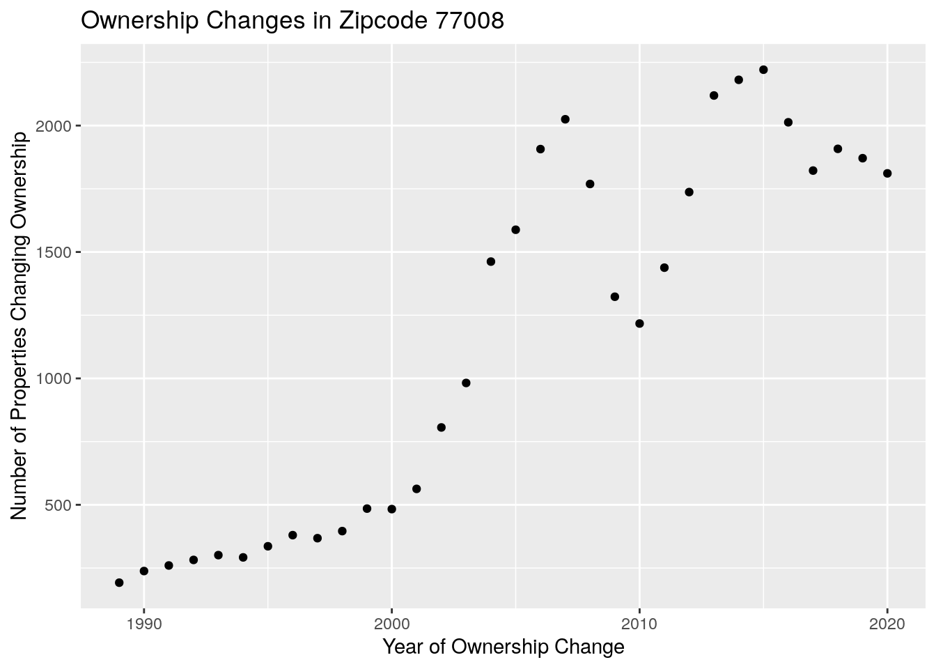
#  Number of unique single family residential addresses per year

Unique_adds <- df %>%
  filter(str_detect(state_class, "A|B")) %>%
  filter(!str_detect(site_addr_1, "^0 ")) %>%
  mutate(yr=lubridate::ymd(paste0(yr,"06-15",sep="-")))

Unique_adds %>%
  group_by(yr, state_class) %>%
  tally() %>%
  #mutate(yr=lubridate::as_date(yr)) %>%
  ggplot(aes(x=yr, y=n, color=state_class)) +
  geom_point() +
  labs(x="Year",
       y="Number of Single-Family Properties",
       title="Density Changes in Zipcode 77008")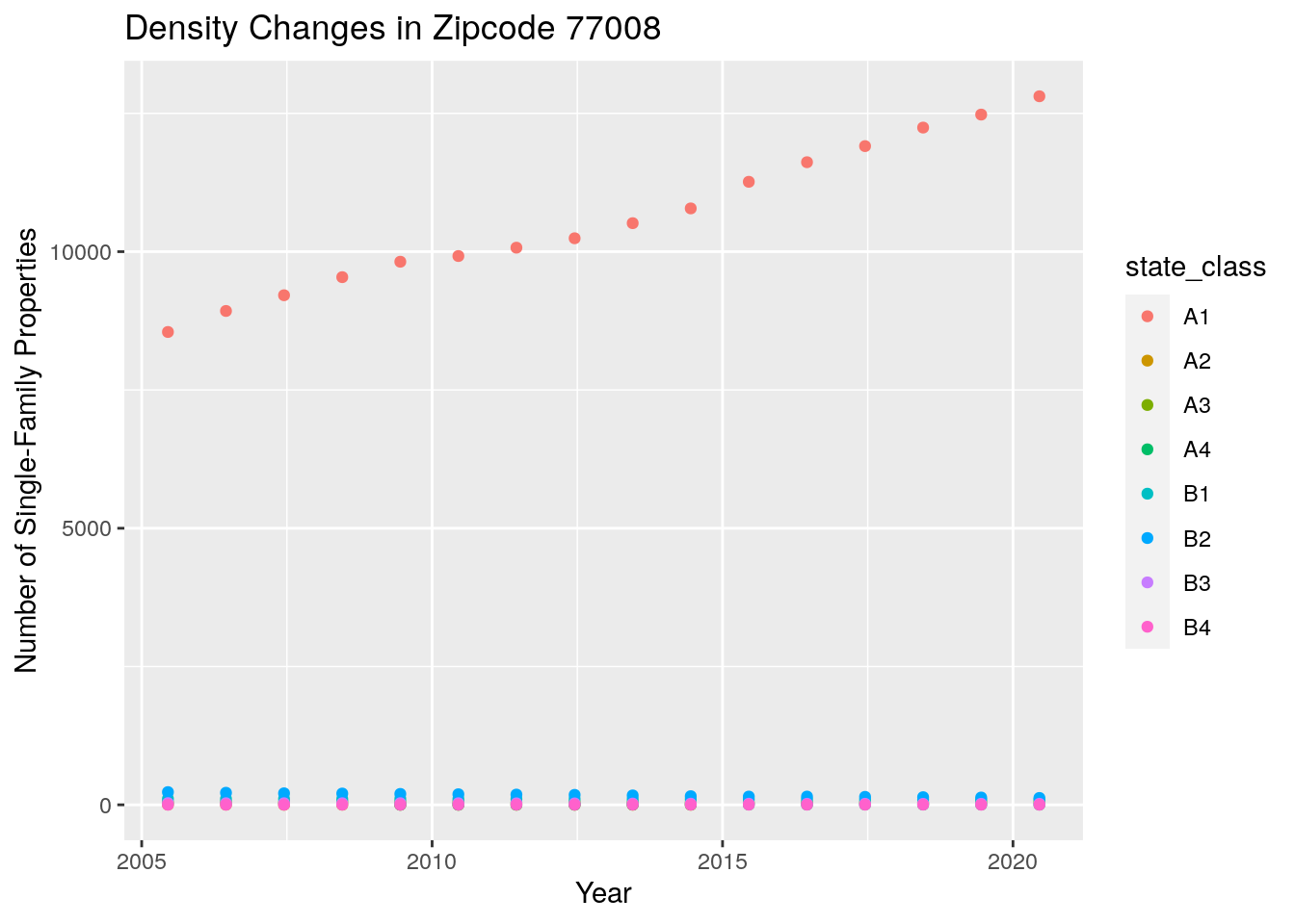
#   A1 houses that have expanded building area

Changes <- df %>%
  filter(state_class=="A1") %>%
  filter(!str_detect(site_addr_1, "^0 ")) %>%
  mutate(yr=lubridate::ymd(paste0(yr,"06-15",sep="-"))) %>%
  arrange(yr) %>%
  group_by(site_addr_1) %>%
    summarize(Beg_yr=first(yr),
              End_yr=last(yr),
              Beg_area=first(bld_ar),
              End_area=last(bld_ar),
              Beg_land=first(land_val),
              End_land=last(land_val),
              Beg_bldg=first(bld_val),
              End_bldg=last(bld_val),
              Beg_appr=first(tot_appr_val),
              End_appr=last(tot_appr_val))

#   Building area changes

Changes %>%
  filter(Beg_yr=="2005-06-15",
         End_yr=="2020-06-15") %>% # Look only at houses that didn't split
  mutate(Area_change = End_area-Beg_area) %>%
  ggplot(aes(x=Area_change)) +
    geom_histogram() +
    labs(x="Change in House Area (Sq-Ft)",
         y="Number of Houses",
         title="Floorspace Changes from 2005-2020 in Zip 77008")
## `stat_bin()` using `bins = 30`. Pick better value with `binwidth`.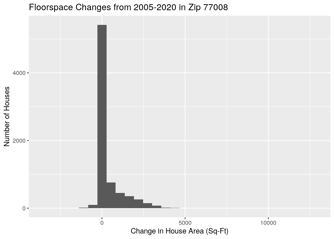
#   Appraisal changes

 Changes %>%
  filter(Beg_yr=="2005-06-15",
         End_yr=="2020-06-15") %>% # Look only at houses that didn't split
  mutate(Appr_change = End_bldg-Beg_bldg) %>%
  ggplot(aes(x=Appr_change)) +
    geom_histogram() +
    labs(x="Change in House Appraisal (dollars)",
         y="Number of Houses",
         title="Appraisal Changes from 2005-2020 in Zip 77008",
         subtitle="Building Value Only")
## `stat_bin()` using `bins = 30`. Pick better value with `binwidth`.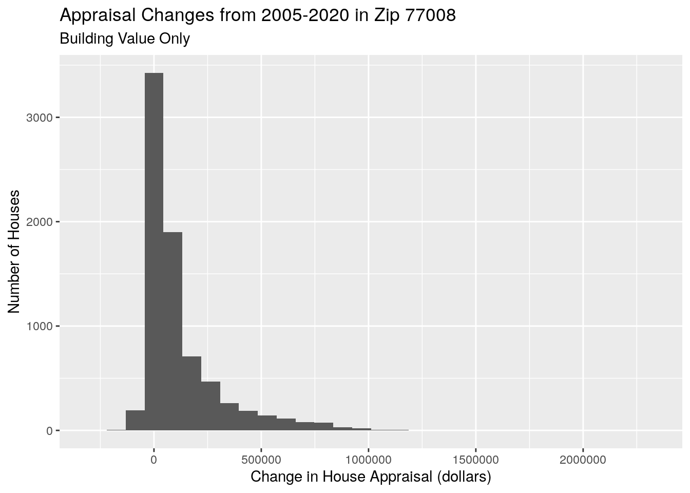
#   Appraisal changes per sq ft

 Changes %>%
  filter(Beg_yr=="2005-06-15",
         End_yr=="2020-06-15") %>% # Look only at houses that didn't split
  mutate(Appr_change = (End_bldg/End_area-Beg_bldg/Beg_area)) %>%
  ggplot(aes(x=Appr_change)) +
    geom_histogram() +
    labs(x="Change in House Appraisal (dollars per square foot)",
         y="Number of Houses",
         title="Appraisal Changes from 2005-2020 in Zip 77008",
         subtitle="Building Value Only")
## `stat_bin()` using `bins = 30`. Pick better value with `binwidth`.## Warning: Removed 5 rows containing non-finite values (stat_bin).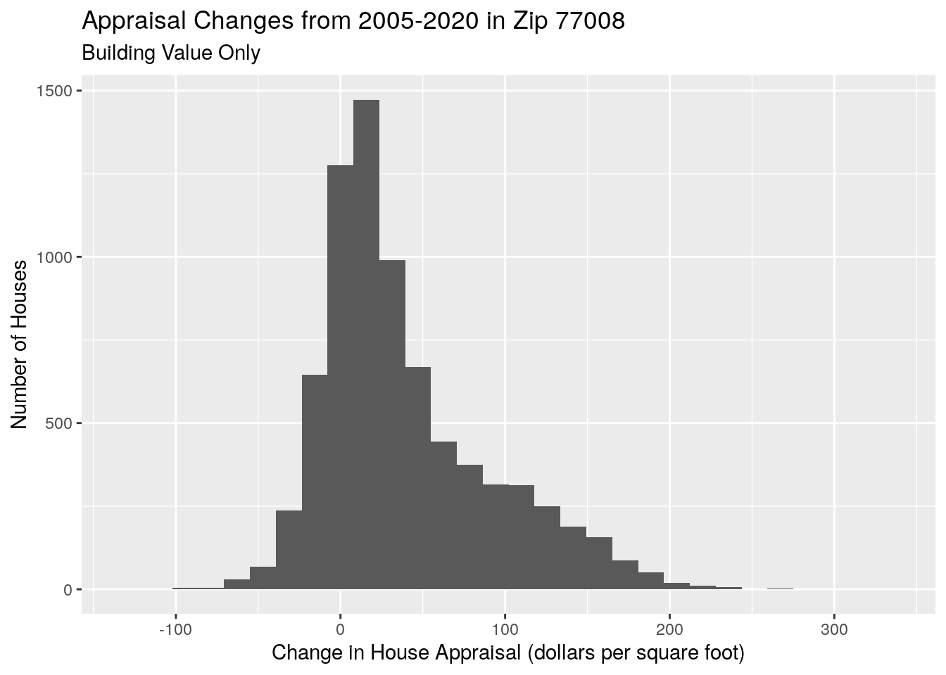
#   Appraisal per sq ft

 Changes %>%
  filter(Beg_yr=="2005-06-15",
         End_yr=="2020-06-15") %>% # Look only at houses that didn't split
  mutate(Appr_psqft = (End_bldg/End_area)) %>%
  ggplot(aes(x=Appr_psqft)) +
    geom_histogram() +
    labs(x="House Appraisal (dollars per square foot)",
         y="Number of Houses",
         title="Appraisal per square foot in 2020 in Zip 77008",
         subtitle="Building Value Only")
## `stat_bin()` using `bins = 30`. Pick better value with `binwidth`.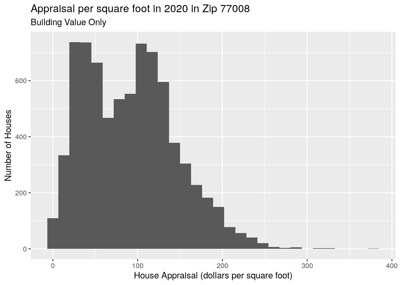
#   Appraisal per sq ft

 foo <-
 Changes %>%
  filter(Beg_yr=="2005-06-15",
         End_yr=="2020-06-15") %>% # Look only at houses that didn't split
  mutate(Appr_psqft_beg = (Beg_bldg/Beg_area)) %>%
  mutate(Appr_psqft_end = (End_bldg/End_area)) %>%
   filter(Beg_area==End_area)

 Changes %>%
  filter(Beg_yr=="2005-06-15",
         End_yr=="2020-06-15") %>% # Look only at houses that didn't split
  mutate(Appr_psqft_beg = (Beg_bldg/Beg_area)) %>%
  mutate(Appr_psqft_end = (End_bldg/End_area)) %>%
   filter(Beg_area==End_area) %>%
   select(Appr_psqft_beg, Appr_psqft_end) %>%
   filter(Appr_psqft_end<350) %>%
   pivot_longer(everything(),
                names_to="group",
                values_to="Psqft") %>%
  ggplot(aes(x=Psqft, fill=group)) +
    geom_histogram(alpha=0.2, position="identity") +
   scale_fill_discrete(labels = c("2005", "2020"),
                       name="Year") +
    labs(x="House Appraisal (dollars per square foot)",
         y="Number of Houses",
         title="Appraisal per sq-ft in 2005 and 2020 in Zip 77008",
         subtitle="Building Value Only, No sq-ft changes")
## `stat_bin()` using `bins = 30`. Pick better value with `binwidth`.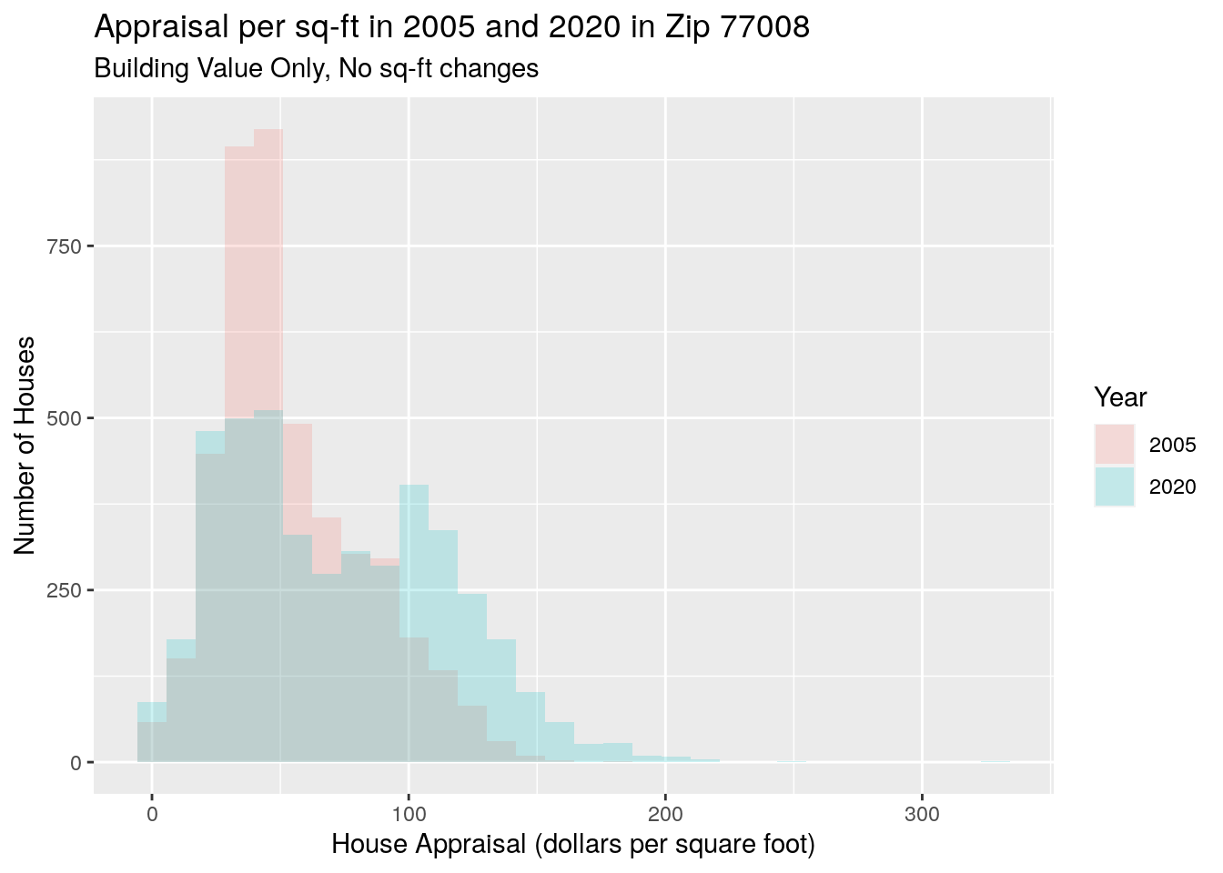
# Changes in building appraisal vs land appraisal
df %>%
mutate(year=lubridate::year(new_own_dt)) %>%
group_by(site_addr_1) %>%
arrange(year) %>%
mutate(Beg_area=first(bld_ar),
End_area=last(bld_ar)) %>%
ungroup() %>%
filter(Beg_area==End_area) %>% # Look only at houses that stayed same size
mutate(Appr_bld = (bld_val/Beg_area)) %>%
mutate(Appr_land = (land_val/land_ar)) %>%
select(Appr_bld, Appr_land, year, Beg_area, land_ar) %>%
filter(Beg_area<land_ar) %>%
filter(!is.nan(Appr_bld)) %>%
filter(Beg_area>0) %>%
filter(Appr_land>0) %>%
filter(Appr_bld>0) %>%
filter(year>1987) %>%
group_by(year) %>%
summarise(mean_bld=mean(Appr_bld),
med_bld=median(Appr_bld),
sd_bld=sd(Appr_bld),
mean_lot=mean(Appr_land),
med_lot=median(Appr_land),
sd_lot=sd(Appr_land)) %>%
pivot_longer(!year,
names_to=c("Statistic", "Type"),
names_sep="_",
values_to="Appraisal") %>%
pivot_wider(names_from="Statistic", values_from="Appraisal") %>%
mutate(Type=ifelse(Type=="bld", "Building", "Lot")) %>%
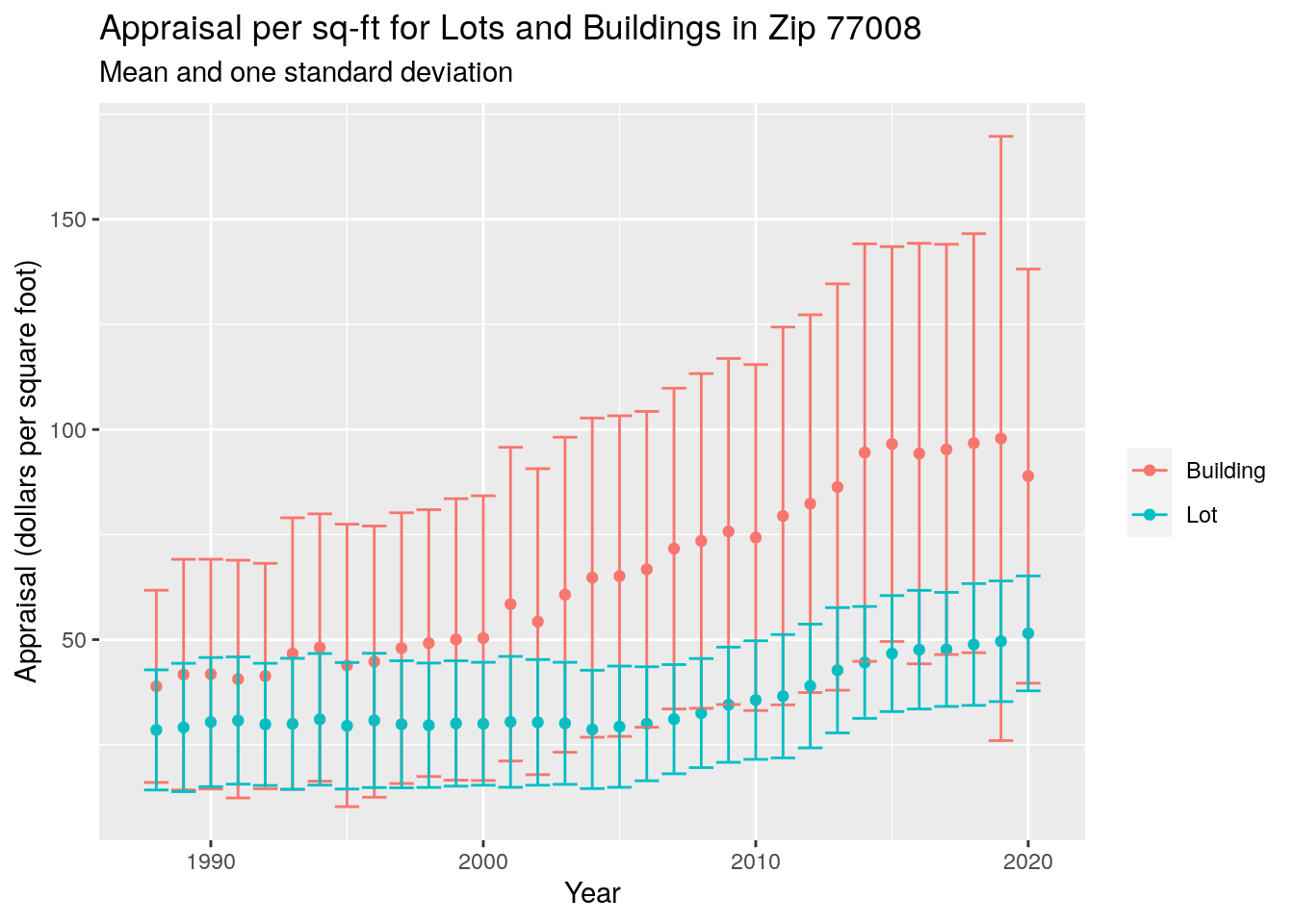
ggplot(aes(x=year, color=Type)) +
geom_point(aes(y=mean)) +
geom_errorbar(aes(ymin=mean-sd, ymax=mean+sd))+
scale_fill_discrete(labels = c("Building", "Lot"),
name="") +
labs(y="Appraisal (dollars per square foot)",
x="Year",
title="Appraisal per sq-ft for Lots and Buildings in Zip 77008",
subtitle="Mean and one standard deviation",
color="")